How do the cell type distributions vary in bulk RNA samples across my variable of interest?
For example, are beta cell proportions different in the pancreas data from diabetes and healthy patients?
Objectives:
Apply the MuSiC deconvolution to samples and compare the cell type distributions
Compare the results from analysing different types of input, for example, whether combining disease and healthy references or not yields better results
The goal of this tutorial is to apply bulk RNA deconvolution techniques to a problem with multiple variables - in this case, a model of diabetes is compared with its healthy counterparts. All you need to compare inferred cell compositions are well-annotated, high quality reference scRNA-seq datasets, transformed into MuSiC-friendly Expression Set objects, and your bulk RNA-samples of choice (also transformed into MuSiC-friendly Expression Set objects). For more information on how MuSiC works, you can check out their github site MuSiC or published article (Wang et al. 2019).
Comment: Research question
How does variable X impact the cell distributions in my samples?
Needs: scRNA-seq reference dataset; bulk RNA-seq samples of interest to compare
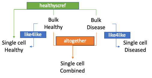
In the standard MuSiC tutorial, we used human pancreas data. We will now use the same single cell reference dataset Segerstolpe et al. 2016 with its 10 samples of 6 healthy subjects and 4 with Type-II diabetes (T2D), as well as the bulk RNA-samples from the same lab (3 healthy, 4 diseased). Both of these datasets were accessed from the public EMBL-EBI repositories and transformed into Expression Set objects in the previous two tutorials. For both the single cell reference and the bulk samples of interest, you have generated Expression Set objects with only T2D samples, only healthy samples, and a final everything-combined sample for the scRNA reference. We won’t need the combined bulk RNA dataset. The plan is to analyse this data in three ways: using a combined reference (altogether); using only the healthy single cell reference (healthyscref); or using a healthy and combined reference separately (like4like), all to identify differences in cellular composition.
If you have followed the previous tutorials, you will have built your single cell ESet object and your bulk ESet object, then you can copy these into a new history now. Otherwise, follow the steps below to import the datasets you’ll need.
There 3 ways to copy datasets between histories
From the original history
Click on the galaxy-gear icon which is on the top of the list of datasets in the history panel
Click on Copy Datasets
Select the desired files
Give a relevant name to the “New history”
Validate by ‘Copy History Items’
Click on the new history name in the green box that have just appear to switch to this history
Using the galaxy-columnsShow Histories Side-by-Side
Click on the galaxy-dropdown dropdown arrow top right of the history panel (History options)
Click on galaxy-columnsShow Histories Side-by-Side
If your target history is not present
Click on ‘Select histories’
Click on your target history
Validate by ‘Change Selected’
Drag the dataset to copy from its original history
Drop it in the target history
From the target history
Click on User in the top bar
Click on Datasets
Search for the dataset to copy
Click on its name
Click on Copy to current History
Get data
Hands On: Data upload
Create a new history for this tutorial “Deconvolution: Compare”
Click galaxy-uploadUpload at the top of the activity panel
Select galaxy-wf-editPaste/Fetch Data
Paste the link(s) into the text field
Press Start
Close the window
Rename the datasets as needed
Add to each file a tag corresponding to #bulk and #scrna
Datasets can be tagged. This simplifies the tracking of datasets across the Galaxy interface. Tags can contain any combination of letters or numbers but cannot contain spaces.
To tag a dataset:
Click on the dataset to expand it
Click on Add Tagsgalaxy-tags
Add tag text. Tags starting with # will be automatically propagated to the outputs of tools using this dataset (see below).
Press Enter
Check that the tag appears below the dataset name
Tags beginning with # are special!
They are called Name tags. The unique feature of these tags is that they propagate: if a dataset is labelled with a name tag, all derivatives (children) of this dataset will automatically inherit this tag (see below). The figure below explains why this is so useful. Consider the following analysis (numbers in parenthesis correspond to dataset numbers in the figure below):
a set of forward and reverse reads (datasets 1 and 2) is mapped against a reference using Bowtie2 generating dataset 3;
dataset 3 is used to calculate read coverage using BedTools Genome Coverageseparately for + and - strands. This generates two datasets (4 and 5 for plus and minus, respectively);
datasets 4 and 5 are used as inputs to Macs2 broadCall datasets generating datasets 6 and 8;
datasets 6 and 8 are intersected with coordinates of genes (dataset 9) using BedTools Intersect generating datasets 10 and 11.
Now consider that this analysis is done without name tags. This is shown on the left side of the figure. It is hard to trace which datasets contain “plus” data versus “minus” data. For example, does dataset 10 contain “plus” data or “minus” data? Probably “minus” but are you sure? In the case of a small history like the one shown here, it is possible to trace this manually but as the size of a history grows it will become very challenging.
The right side of the figure shows exactly the same analysis, but using name tags. When the analysis was conducted datasets 4 and 5 were tagged with #plus and #minus, respectively. When they were used as inputs to Macs2 resulting datasets 6 and 8 automatically inherited them and so on… As a result it is straightforward to trace both branches (plus and minus) of this analysis.
Altogether: Deconvolution with a combined sc reference
Tools are frequently updated to new versions. Your Galaxy may have multiple versions of the same tool available. By default, you will be shown the latest version of the tool. This may NOT be the same tool used in the tutorial you are accessing. Furthermore, if you use a newer tool in one step, and try using an older tool in the next step… this may fail! To ensure you use the same tool versions of a given tutorial, use the Tutorial mode feature.
Open your Galaxy server
Click on the curriculum icon on the top menu, this will open the GTN inside Galaxy.
Navigate to your tutorial
Tool names in tutorials will be blue buttons that open the correct tool for you
Note: this does not work for all tutorials (yet)
You can click anywhere in the grey-ed out area outside of the tutorial box to return back to the Galaxy analytical interface
Warning: Not all browsers work!
We’ve had some issues with Tutorial mode on Safari for Mac users.
Try a different browser if you aren’t seeing the button.
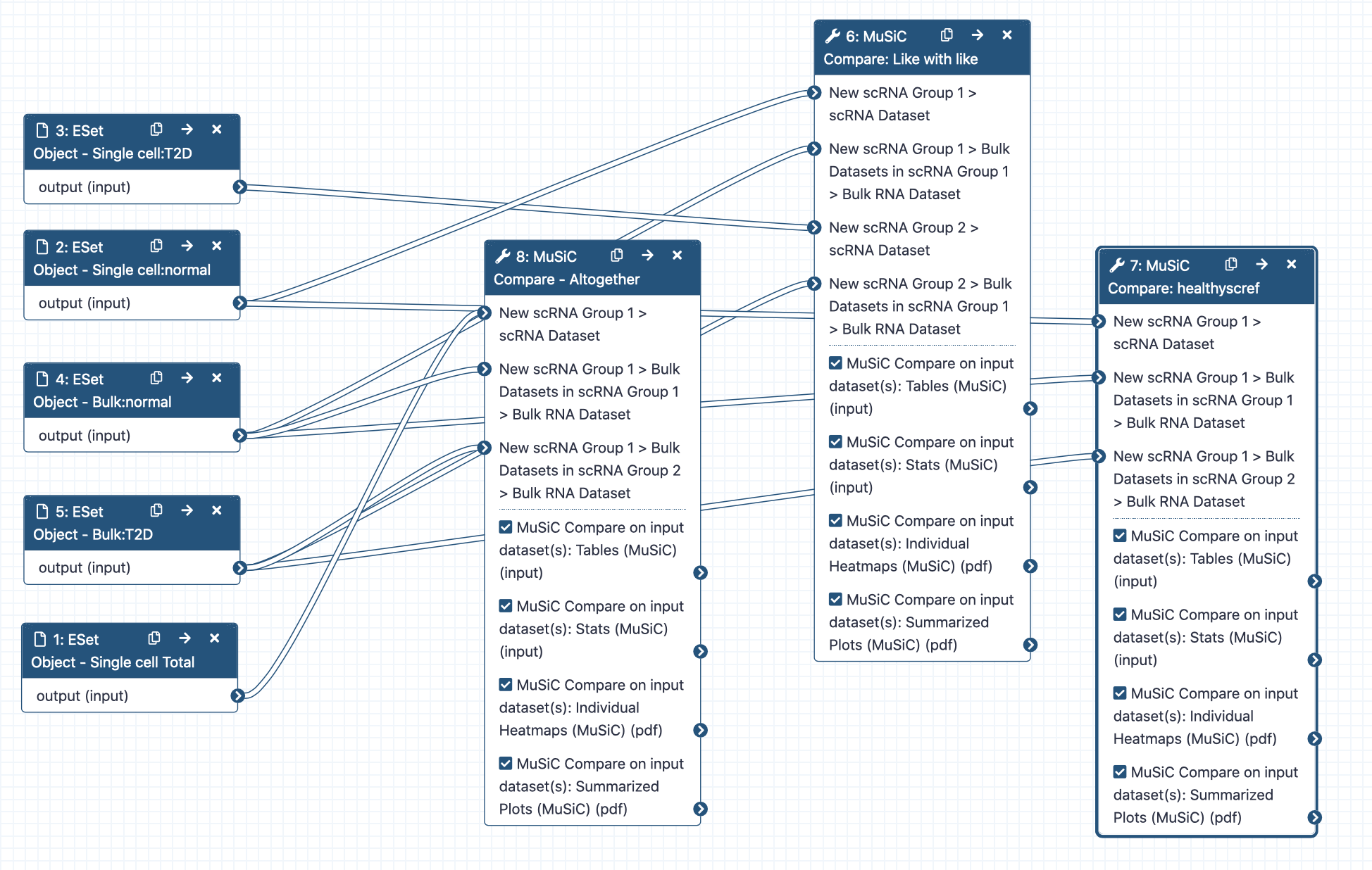
Hands On: Comparing: altogether
MuSiC Compare ( Galaxy version 0.1.1+galaxy4) with the following parameters:
Summarised Plots <- This is the most interesting output, because it has the pretty pictures!
Individual Heatmaps <- This kind of does what standard (non-Comparing) MuSiC does for each sample, rather than combining them.
Stats <- This will be very handy if you want to make any statistical calculations, as it contains medians and quartiles
Tables <- This contains the cell proportions found within each sample as well as the number of reads.
Summarised Plots
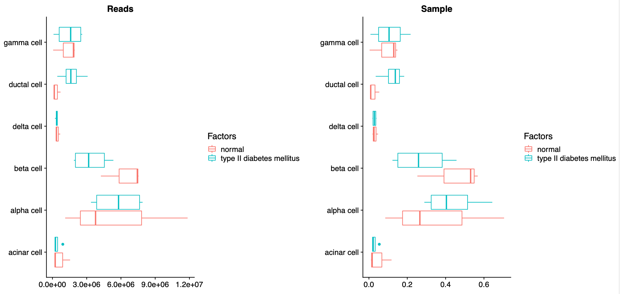
Examine galaxy-eye the output file Summarised Plots (MuSiC). Now the first few pages are similar to the standard deconvolution tool, but now comparing across the factor of interest (disease). Among the myriad of visualisations available, our favourite is on page 5 - a comparison of inferred cell proportions across disease.
Here we can see that the bulk-RNA seq samples from the T2D patients contain markedly fewer beta cells as compared with their healthy counterparts. This makes sense, so that’s good!
Individual Heatmaps
Examine galaxy-eye the output file Individual heatmaps (MuSiC). This shows the cell distribution across each of the individual samples, separated out by disease factor into two separate plots, but ultimately isn’t particularly informative.
If you select the Stats dataset, you’ll find it contains four sets of data, Bulk_disease: Read Props, Bulk_disease: Sample Props, Bulk_healthy: Read Props and Bulk_healthy: Sample Props. Examine galaxy-eye the file Bulk_disease: Sample Props. This contains summary statistics (Min, quartiles, median, mean, etc.) for each phenotype. This could be quite helpful if you’re trying to statistically identify differences across samples.
Finally, if you select the Tables dataset, you’ll find it contains three sets of data, Data Table, Matrix of Cell Type Read Counts, and Matrix of Cell Type Sample Proportions.
Examine galaxy-eye the file Data Table. This contains the inferred proportions and reads associated with each sample and cell type, along with its important factor of interest (Disease). In this tutorial, we tend to use sample proportions rather than read count, but either works. The two other matrix files are just portions of this data table.
Overall, our interpretation here is that the differences are less pronounced. It’s interesting to conjecture whether this is an artefact of analysis, or whether - possibly - the beta cells in the diseased samples are not only fewer, but also contain fewer beta-cell specific transcripts (and thereby inhibited beta cell function), thereby lowering the bar for the inference of a beta cell and leading to a higher proportion of interred B-cells.
Let’s try one more inference - this time, we’ll use only healthy cells as a reference, to (theoretically) make a more consistent analysis across the two phenotypes.
healthyscref: Deconvolution using only healthy cells as a reference
Hands On: Healthy sc reference only inference
MuSiC Compare ( Galaxy version 0.1.1+galaxy4) with the following parameters:
If using a like4like inference reduced the difference between the phenotype, aligning both phenotypes to the same (healthy) reference exacerbated them - there are even fewer beta cells in the output of this analysis.
Overall, it’s important to remember how the inference changes depending on the reference used - for example, a combined reference might have majority healthy samples or diseased samples, so that would impact the inferred cellular compositions.
Conclusion
Congrats! You’ve made it to the end of this suite of deconvolution tutorials! You’ve learned how to find quality data for reference and for analysis, how to reformat it for deconvolution using MuSiC, and how to compare cellular inferences using multiple kinds of reference datasets. You can find the workflow for this tutorial and an example history.
We also post new tutorials / workflows there from time to time, as well as any other news.
point-right If you’d like to contribute ideas, requests or feedback as part of the wider community building single-cell and spatial resources within Galaxy, you can also join our Single cell & sPatial Omics Community of Practice.
Further information, including links to documentation and original publications, regarding the tools, analysis techniques and the interpretation of results described in this tutorial can be found here.
References
Segerstolpe, Å., A. Palasantza, P. Eliasson, E.-M. Andersson, A.-C. Andréasson et al., 2016 Single-cell transcriptome profiling of human pancreatic islets in health and type 2 diabetes. Cell metabolism 24: 593–607. 10.1016/j.cmet.2016.08.020
Wang, X., J. Park, K. Susztak, N. R. Zhang, and M. Li, 2019 Bulk tissue cell type deconvolution with multi-subject single-cell expression reference. Nature communications 10: 1–9. 10.1038/s41467-018-08023-x
Did you use this material as an instructor? Feel free to give us feedback on how it went.
Did you use this material as a learner or student? Click the form below to leave feedback.
Hiltemann, Saskia, Rasche, Helena et al., 2023 Galaxy Training: A Powerful Framework for Teaching! PLOS Computational Biology 10.1371/journal.pcbi.1010752
Batut et al., 2018 Community-Driven Data Analysis Training for Biology Cell Systems 10.1016/j.cels.2018.05.012
@misc{single-cell-bulk-music-4-compare,
author = "Wendi Bacon and Mehmet Tekman",
	title = "Comparing inferred cell compositions using MuSiC deconvolution (Galaxy Training Materials)",
	year = "",
	month = "",
	day = "",
	url = "\url{https://training.galaxyproject.org/training-material/topics/single-cell/tutorials/bulk-music-4-compare/tutorial.html}",
	note = "[Online; accessed TODAY]"
}
@article{Hiltemann_2023,
	doi = {10.1371/journal.pcbi.1010752},
	url = {https://doi.org/10.1371%2Fjournal.pcbi.1010752},
	year = 2023,
	month = {jan},
	publisher = {Public Library of Science ({PLoS})},
	volume = {19},
	number = {1},
	pages = {e1010752},
	author = {Saskia Hiltemann and Helena Rasche and Simon Gladman and Hans-Rudolf Hotz and Delphine Larivi{\`{e}}re and Daniel Blankenberg and Pratik D. Jagtap and Thomas Wollmann and Anthony Bretaudeau and Nadia Gou{\'{e}} and Timothy J. Griffin and Coline Royaux and Yvan Le Bras and Subina Mehta and Anna Syme and Frederik Coppens and Bert Droesbeke and Nicola Soranzo and Wendi Bacon and Fotis Psomopoulos and Crist{\'{o}}bal Gallardo-Alba and John Davis and Melanie Christine Föll and Matthias Fahrner and Maria A. Doyle and Beatriz Serrano-Solano and Anne Claire Fouilloux and Peter van Heusden and Wolfgang Maier and Dave Clements and Florian Heyl and Björn Grüning and B{\'{e}}r{\'{e}}nice Batut and},
	editor = {Francis Ouellette},
	title = {Galaxy Training: A powerful framework for teaching!},
	journal = {PLoS Comput Biol}
}
Congratulations on successfully completing this tutorial!
Do you want to extend your knowledge?
Follow one of our recommended follow-up trainings:
Questions:
 Open image in new tab

 Open image in new tab
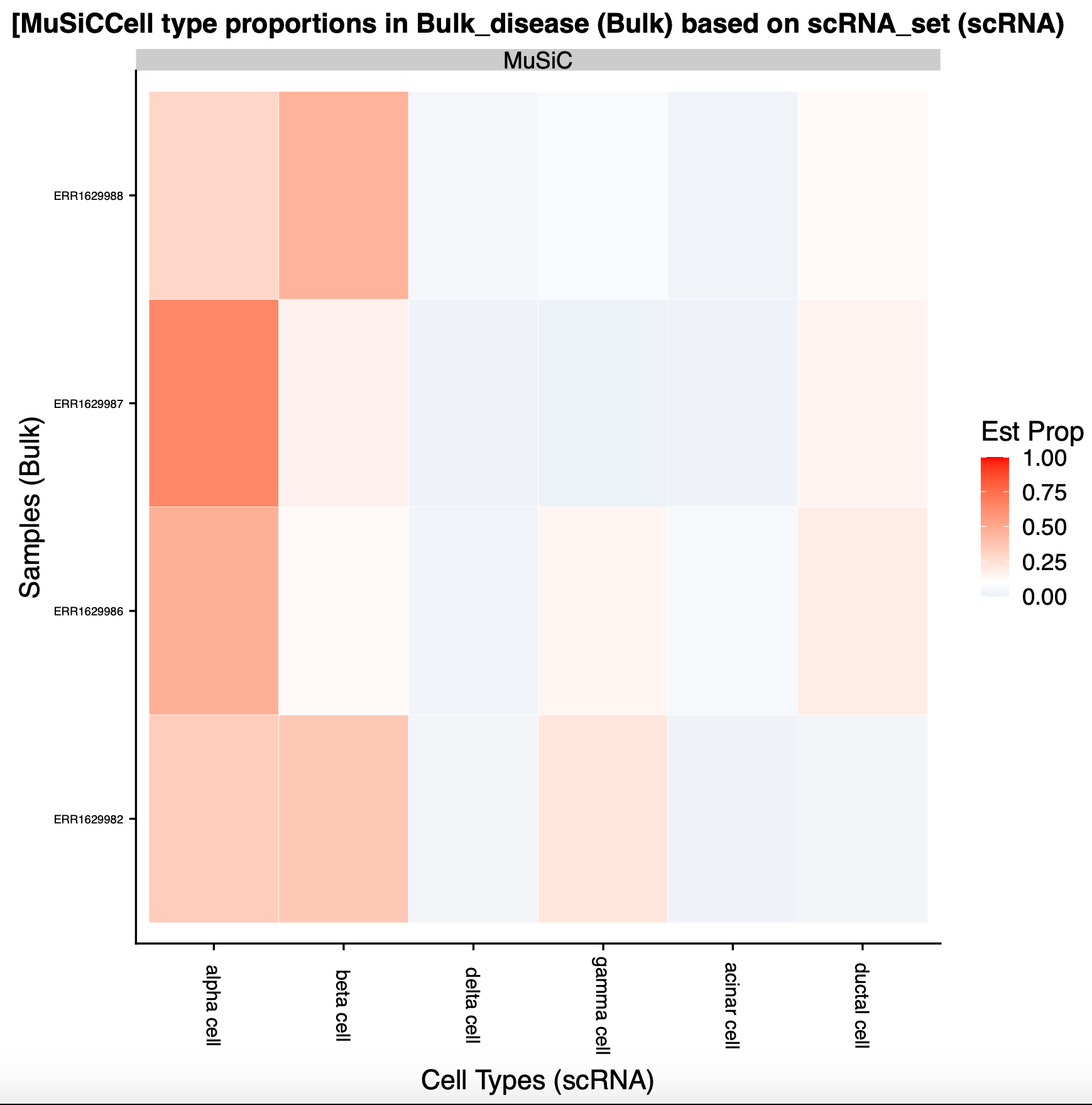 Open image in new tab
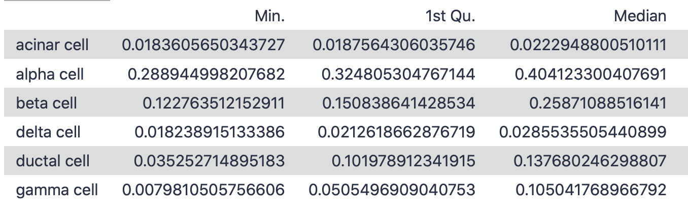 Open image in new tab
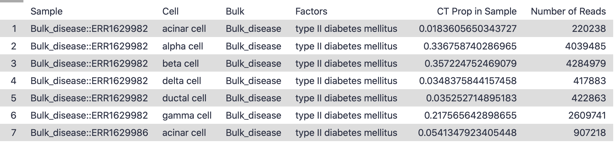 Open image in new tab
Open image in new tab
Open image in new tab
 Open image in new tab