Bulk RNA-seq data contains a mixture of transcript signatures from several types of cells. We wish to deconvolve this mixture to obtain estimates of the proportions of cell types within the bulk sample. To do this, we can use single cell RNA-seq data as a reference for estimating the cell type proportions within the bulk data.
In this tutorial, we will use bulk and single-cell RNA-seq data, including matrices of similar tissues from different sources, to illustrate how to infer cell type abundances from bulk RNA-seq.
The heterogeneity that exists in the cellular composition of bulk RNA-seq can add bias to the results from differential expression analysis. In order to circumvent this limitation, RNA-seq deconvolution aims to infer cell type abundances by modelling the gene expressions levels as ‘weighted sums’ of cell type specific expression profiles.
So… You fancy some maths do you? Good! This is important, as you’ll see variations of the phrase ‘weighted sums’ if you ever look at any papers in the field! Let’s think about just the ‘sums’ here.
If we think about the total expression of a given gene you might get from bulk RNA-seq, you could also think about it as the sum of the expression of each cell, for example,
Total = cella expression + cellb expression … (and so forth)
This is a ‘sum’, because we’re adding up all the cells. If we now think about how we expect similar expression from similar cell types, we could change this to the following:
Total = cell_typea expression + cell_typeb expression … (and so forth)
BUT WAIT! That’s not strictly true, because the cell types are not all in equal proportion (if only!). So we have to take into account another variable, the proportion a given cell type takes up in a sample. So we now have:
Total = Proportiona x cell_typea expression + Proportionb x cell_typeb expression
So now, we are using the sums of expression based off of the cell proportion. And if you’re a mathematician, you might instead put this as
T = C x P
or some fancier formulas…(read more in-depth here if you like!)
The point is, if we have an idea of what the average expression should be for each gene (what we can get from single cell RNA-seq data, C), and we have the total expression (from the bulk RNA-seq, T), then we can infer the cell proportions (P).
Many different computational methods have been developed to estimate these cell type proportions, but in this tutorial we will be using the MuSiC tool suite (Wang et al. 2019) to estimate the proportion of individual cell types in our bulk RNA-seq datasets.
MusiC
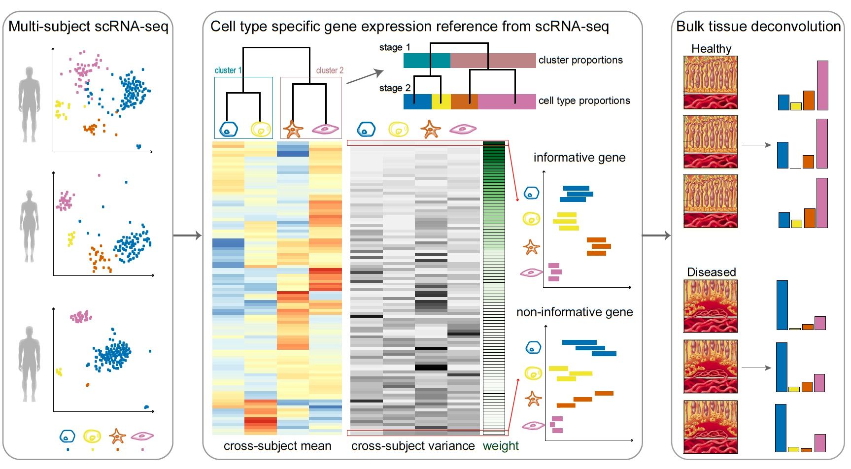
MuSiC uses cell-type specific gene expression from single-cell RNA seq data to characterize cell type compositions (proportions) from bulk RNA-seq data in complex tissues. By appropriate weighting of genes showing cross-subject (sample to sample) and cross-cell (cells of the same cell type within a sample) consistency, MuSiC enables the transfer of cell type-specific gene expression information from one dataset to another.
Question
What is a weighted sum? Hint: What kinds of genes would be best for distinguishing cell types, and what kinds of genes would make it difficult?
So you know what the Sum is from above - the total expression of a given gene in a bulk RNA-seq sample depends on the proportion of cell types and the average expression level of each of those cell types (T = C x P). However, single cell RNA-seq data is highly variable. Cell-type specific expression in genes with lower variation from sample to sample (i.e. person to person or organism to organism) and cell to cell (i.e. within a sample) will be the most useful for distinguishing cells, while genes that vary heavily (i.e. high in cell typea in one sample, but low in cell typea in another sample) will be the least useful in accurately distinguishing cells. Therefore, to accurately use the mean expression level in a cell_type, MusiC weights the sums, favouring more consistently expressed genes in cell types.
Solid tissues often contain closely related cell types that are difficult to distinguish from one another, a phenomenon known as “collinearity”. To deal with collinearity, MuSiC can also employ a tree-guided procedure that recursively zooms in on closely related cell types. Briefly, MuSic first groups similar cell types into the same cluster and estimates cluster proportions, then recursively repeats this procedure within each cluster.
Here we will extract cell proportions from a bulk data of human pancreas data from Fadista et al. 2014 concerning 56 638 genes across 89 samples, using a single cell human pancreas dataset from Segerstolpe et al. 2016 containing 25 453 genes across 2209 cells, clustered into 14 cell types, from 6 healthy subjects and 4 with Type-II diabetes (T2D). If the deconvolution is good, and the datasets are compatible with sufficient enough overlap, we should be able to identify the same cell types from the bulk data.
Get data
Hands On: Data upload
Create a new history for this tutorial “Deconvolution: Cell Type inference of Human Pancreas Data”
Import the files from Zenodo or from
the shared data library (GTN - Material -> single-cell
-> Bulk RNA Deconvolution with MuSiC):
Click galaxy-uploadUpload at the top of the activity panel
Select galaxy-wf-editPaste/Fetch Data
Paste the link(s) into the text field
Press Start
Close the window
As an alternative to uploading the data from a URL or your computer, the files may also have been made available from a shared data library:
Go into Libraries (left panel)
Navigate to the correct folder as indicated by your instructor.
On most Galaxies tutorial data will be provided in a folder named GTN - Material –> Topic Name -> Tutorial Name.
Select the desired files
Click on Add to Historygalaxy-dropdown near the top and select as Datasets from the dropdown menu
In the pop-up window, choose
“Select history”: the history you want to import the data to (or create a new one)
Click on Import
Rename the datasets
Check the datatype
Click on the galaxy-pencilpencil icon for the dataset to edit its attributes
In the central panel, click galaxy-chart-select-dataDatatypes tab on the top
In the galaxy-chart-select-dataAssign Datatype, select tabular from “New Type” dropdown
Tip: you can start typing the datatype into the field to filter the dropdown menu
Click the Save button
Add to each expression file a tag corresponding to #bulk and #scrna
Datasets can be tagged. This simplifies the tracking of datasets across the Galaxy interface. Tags can contain any combination of letters or numbers but cannot contain spaces.
To tag a dataset:
Click on the dataset to expand it
Click on Add Tagsgalaxy-tags
Add tag text. Tags starting with # will be automatically propagated to the outputs of tools using this dataset (see below).
Press Enter
Check that the tag appears below the dataset name
Tags beginning with # are special!
They are called Name tags. The unique feature of these tags is that they propagate: if a dataset is labelled with a name tag, all derivatives (children) of this dataset will automatically inherit this tag (see below). The figure below explains why this is so useful. Consider the following analysis (numbers in parenthesis correspond to dataset numbers in the figure below):
a set of forward and reverse reads (datasets 1 and 2) is mapped against a reference using Bowtie2 generating dataset 3;
dataset 3 is used to calculate read coverage using BedTools Genome Coverageseparately for + and - strands. This generates two datasets (4 and 5 for plus and minus, respectively);
datasets 4 and 5 are used as inputs to Macs2 broadCall datasets generating datasets 6 and 8;
datasets 6 and 8 are intersected with coordinates of genes (dataset 9) using BedTools Intersect generating datasets 10 and 11.
Now consider that this analysis is done without name tags. This is shown on the left side of the figure. It is hard to trace which datasets contain “plus” data versus “minus” data. For example, does dataset 10 contain “plus” data or “minus” data? Probably “minus” but are you sure? In the case of a small history like the one shown here, it is possible to trace this manually but as the size of a history grows it will become very challenging.
The right side of the figure shows exactly the same analysis, but using name tags. When the analysis was conducted datasets 4 and 5 were tagged with #plus and #minus, respectively. When they were used as inputs to Macs2 resulting datasets 6 and 8 automatically inherited them and so on… As a result it is straightforward to trace both branches (plus and minus) of this analysis.
Figure 2: Peeking at the tabular scRNA expression dataset
Rows correspond to gene names, and columns to cell identifiers
These are the number of reads or counts for each gene for each cell
The data has not been normalised since the counts are integer and not decimal
Single-cell datasets can be very sparse for a variety of reasons relating to dropouts and biological factors. For more information, please see the introduction single-cell RNA-seq slides#41.
Inspect the #bulk expression file
Question
What do the rows and columns correspond to?
In which field is there likely to be overlap with the #scrna dataset?
Figure 3: Peeking at the tabular bulk RNA-seq expression dataset
As before with the #scrna dataset, rows correspond to gene names and columns to sample identifiers.
The sample identifiers and the cell identifiers are completely different, but the gene names appear to be using the same symbols as the #scrna dataset, so the gene field is the common factor here.
Figure 4: Peeking at the tabular scRNA phenotype dataset
The first column is the index column, which uses the cell identifiers in the header of the #scrna expression file, so the phenotypes file describes the cells.
SubjectName tells us whether the cell (on that row) is labelled as Type-II diabetes or not, “Non T2D” or “T2D” respectively.
cellType tells us which cell type the cell was assigned to. This could be the result of prior-clustering and then labelling, or the cells could be labelled before analysis.
Inspect the #bulk phenotype file
Question
Does the phenotypes file describe genes or samples?
Is the SubjectName field related to the SubjectName field in the #scrna phenotypes file?
What other factors are in the phenotypes file?
Is the tissue field related to the cellType field in the #scrna phenotypes file?
Figure 5: Peeking at the tabular bulk RNA-seq phenotype dataset
The first column is the index column, which uses the sample identifiers in the header of the #bulk expression file, so the phenotypes file describes the samples.
The SubjectName column uses a completely different set of identifiers from the #scrna phenotypes file so they should be assumed to be unrelated.
We see age, bmi, hba1c, gender, tissue. HbA1c appears to be a gene of interest related to a known phenotype.
This is the question we wish to answer in the deconvolution. Visually, there appears to be no overlap, but the “pancreatic islets” tissue likely consists of several cell types that show expressions profiles with some affinity to the single cell types described in the #scrna phenotypes file.
The bulk RNA-seq phenotype file lists the main factors of interest, and HbA1c appears to be a specific gene associated with a phenotype. It is well known that the beta cell proportions are related to T2D disease status. In the progress of T2D, the number of beta cells decreases. One of the most important tests for T2D is the HbA1c (hemoglobin A1c) test. When the HbA1c level is greater than 6.5%, the patient is diagnosed as T2D. We will look later at the beta cell proportions relationship with HbA1c level in this deconvolution analysis.
Building the Expression Set objects
Tools are frequently updated to new versions. Your Galaxy may have multiple versions of the same tool available. By default, you will be shown the latest version of the tool. This may NOT be the same tool used in the tutorial you are accessing. Furthermore, if you use a newer tool in one step, and try using an older tool in the next step… this may fail! To ensure you use the same tool versions of a given tutorial, use the Tutorial mode feature.
Open your Galaxy server
Click on the curriculum icon on the top menu, this will open the GTN inside Galaxy.
Navigate to your tutorial
Tool names in tutorials will be blue buttons that open the correct tool for you
Note: this does not work for all tutorials (yet)
You can click anywhere in the grey-ed out area outside of the tutorial box to return back to the Galaxy analytical interface
Warning: Not all browsers work!
We’ve had some issues with Tutorial mode on Safari for Mac users.
Try a different browser if you aren’t seeing the button.
For now we need to construct our Expression set objects that will be consumed by MuSiC.
Expression Set objects are a container for high-throughput assays and experimental metadata. The ExpressionSet class is derived from eSet, and requires a matrix named exprs.
The ExpressionSet class is designed to combine several different sources of information into a single convenient structure. An ExpressionSet can be manipulated (e.g., subsetted, copied) conveniently, and is the input or output from many Bioconductor functions.
The data in an ExpressionSet is complicated, consisting of:
expression data (exprs, or assayData; assayData is used to hint at the methods used to access different data components, as we will see below);
metadata describing samples in the experiment (phenoData, pData)
information related to the protocol used for processing each sample and usually extracted from manufacturer files (protocolData);
annotations and metadata about the features on the chip or technology used for the experiment (featureData, annotation, fData);
and a flexible structure to describe the experiment (experimentData).
The ExpressionSet class coordinates all of this data, so that you do not usually have to worry about the details.
An ExpressionSet object has many data slots, the principle of which are the experiment data (exprs), the phenotype data (pData), as well metadata pertaining to experiment information and additional annotations (fData).
Construct Expression Set Object ( Galaxy version 0.1.1+galaxy4) with the following parameters:
We will now inspect these objects we just created to see what information we can extract out of them, and how these multiple datasets are summarized within the object.
Hands On: Inspect and Describe the scRNA ExpressionSet Object
Obtain General Info about the data set
galaxy-eye Click on the #scrnaGeneral Info dataset in the history view (output of Construct Expression Set Objecttool)
Obtain Feature Information about the data set
Inspect Expression Set Object ( Galaxy version 0.1.1+galaxy4) with the following parameters:
Warning: Danger: This tool has needs!
You may need to click the dataset from your history and drag it into the input of this tool. Some browsers don’t allow this.
param-file“ESet Dataset”: #scrna (output of Construct Expression Set Objecttool)
“Inspect”: Feature Data Table
Comment: Features or Genes?
“Features” are synonymous with “Genes” in a genomic setting, but data scientists tend to prefer to use the former term, as it can be used in other non-genomic settings.
By inspecting the Feature Data Table, you should see a list of gene names.
Obtain the dimensions of the data set
Inspect Expression Set Object ( Galaxy version 0.1.1+galaxy4) with the following parameters:
param-file“ESet Dataset”: #scrna (output of Construct Expression Set Objecttool)
“Inspect”: Dimension
Question
How many samples are in the dataset, and how many genes?
Does this agree with the original input tabular expression data set?
1097 samples and 25 453 genes
Yes!
Estimating Cell Type proportions
Instead of selecting marker genes, MuSiC gives weights to each gene. The weighting scheme is based on cross-subject variation, by up-weighing genes with low variation and down-weighing genes with high variation in a cell type. Here we demonstrate this step-by-step with the human pancreas datasets.
The deconvolution of 89 subjects from Fadista et al. 2014 is performed with the bulk data GSE50244 expression set and single cell reference EMTAB. The estimation was constrained on 6 major cell types: alpha, beta, delta, gamma, acinar and ductal, which make up over 90% of the whole islet.
Cell Type estimation with MuSiC
The deconvolution process can be performed by simply inputting the bulk RNA-seq & scRNA-seq datasets and then hitting execute. However, in this section we will be tracing the effect of a disease phenotype across both datasets.
Here we will use one of the factors from the bulk RNA-seq phenotypes related to the T2D disease status. Any bulk RNA-seq sample coming from a patient with the HbA1c factor above 6.5% would be clinically classified as having T2D, so we want to compare these datasets with non-diseased samples. As diabetes affects Beta cells, we’re particularly interested in these cells proportions - mostly to prove that the deconvolution has worked well!
It’s also important that input scRNA-seq datasets (ideally) have some representation of cell populations from diseased patients.
Question
Why should the scRNA-seq dataset contain diseased cells and healthy cells?
For instance, there might be a weird extra cell type that appears in the disease phenotype. Or perhaps there is a missing cell type in the disease phenotype. Without both healthy & diseased datasets, the cells in the bulk datasets might not be fully identifiable. Saying that, such datasets are not always available - something to keep in mind when interpreting the results!
Hands On: Task description
MuSiC ( Galaxy version 0.1.1+galaxy4) with the following parameters:
*MuSiC sometimes does not show up from the tool search box. You may need to look for it under the Single Cell heading
param-file“scRNA Dataset”: #scrna (output of Construct Expression Set Objecttool)
param-file“Bulk RNA Dataset”: #bulk (output of Construct Expression Set Objecttool)
“Purpose”: Estimate Proportions
“Methods to use”: MuSiC and NNLS
“Cell Types Label from scRNA dataset”: cellType
“Samples Identifier from scRNA dataset”: sampleID
“Comma list of cell types to use from scRNA dataset”: alpha,beta,delta,gamma,acinar,ductal
Under “Show proportions of a disease factor?”: Yes
“scRNA Phenotype Cell Target”: beta
“Bulk Phenotype Target”: hba1c (Factor from Bulk Phenotype)
“Bulk Phenotype Target Threshold”: 6.5
“scRNA Sample Disease Group”: T2D (Ideally a Factor from scRNA Phenotype)
“scRNA Sample Disease Group (Scale)”: 5
Comment
It’s important to set a phenotype target threshold, otherwise no cells will be matched for the phenotype target. In this case, when the HbA1c level is greater than 6.5%, the patient is diagnosed as T2D.
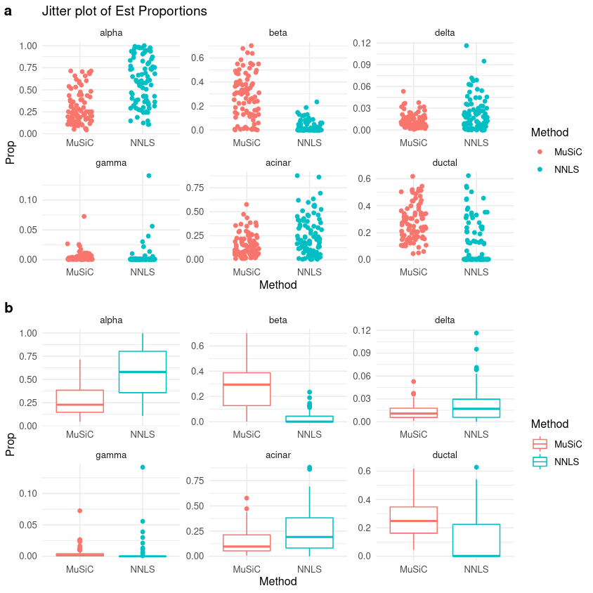
The estimated proportions are normalized such that the proportions of cell types within each sample sum to 1. MuSic compares itself against a previous method of deconvolution known as Non-negative Least-Squares (NNLS), which MuSic supercededs via its Weighted Non-negative Least-Squares (W-NNLS) methodology. You can remove this if you wish from within the tool parameters when running.
In the above image you can see (a) the estimated proportion of cells for each of the 6 declared types, as calculated by MuSiC and the NNLS methods, respectively. In the (b) section, this information is better represented as a box plot to show you the distribution of cell type proportions.
Figure 8: (top) Cell type proportions by disease factor, and (bottom) HbA1c factor expression against beta cell type proportion
As stated previously, it is well known that the beta cell proportions are related to T2D disease status. As T2D progresses, the number of beta cells decreases. In the above image we can see in (a) that we have the same information as previous, but we also distinguish between cells that from patients with T2D status over the Normal cell phenotypes. Section (b) further explores this with a linear regression showing the cell type proportion of cells with HbA1c expression, where we see that there is a significant negative correlation between HbA1c level and beta cell proportions.
Comment
We can extract the coefficients of this fitting by looking at the Log of Music Fitting Data in the Summaries and Logs output collection:
In addition to HbA1c levels, gender has also correlated with beta cell proportions. This is unsurprising, as more men have diabetes than women and sex is known to impact HbA1c levels.
Proportions of Cell Type to each Bulk RNA sample
One question we might wish to ask is: what affinity did each of the 6 single cell types have to each of the 89 subjects in the bulk data? For this we can look at the raw data galaxy-eyeMuSiC Estimated Proportions of Cell Types in the Proportion Matrices, to get a glimpse of cell type compositions on a bulk RNA sample level.
Both the MuSiC and the NNLS calculations of this data is best represented in the below heatmap, with RNA samples as rows and cell types as columns:
Figure 9: Heatmap of cell type proportions at the RNA sample level.
Question
Which cell types are under-represented in the NNLS method?
Which cell types do not appear to be present in both?
Here it is evident that the previous NNLS method over-represents the Alpha cell type compared to the MuSiC method which gives more weight to the Beta and Ductal cell types, which were under-represented in the NNLS method.
The Delta and Gamma cell types appear empty in both.
Estimation of cell type proportions with pre-grouping of cell types
In the previous section we estimated cell types under the assumption that that the gene expression between cell types was largely independent. However, solid tissues often contain closely related cell types. This correlation of gene expression between these cell types is termed ‘collinearity’, which makes it difficult to resolve their relative proportions in bulk data.
To deal with collinearity, MuSiC can also employ a tree-guided procedure that recursively zooms in on closely related cell types.
Briefly, similar cell types are grouped into the same cluster and their cluster proportions are estimated, then this procedure is recursively repeated within each cluster. At each recursion stage, only genes that have low within-cluster variance are used, as they should be consistent within a cell type. This is critical as the mean expression estimates of genes with high variance are affected by the pervasive bias in cell capture of scRNA-seq experiments, and thus cannot serve as reliable reference.
To perform this analysis, we will use mouse kidney single-cell RNA-seq data from Park et al. 2018 described by 16 273 genes over a trimmed subset of 10 000 cells, giving 16 unique cell type (2 of which are novel) across 7 subjects. The bulk RNA-seq dataset is from Beckerman et al. 2017 and contains mouse kidney tissue described by 19 033 genes over 10 samples.
Get data
Hands On: Data upload
Create a new history for this tutorial “Deconvolution: Dendrogram of Mouse Data”
Import the files from Zenodo or from
the shared data library (GTN - Material -> single-cell
-> Bulk RNA Deconvolution with MuSiC):
Click galaxy-uploadUpload at the top of the activity panel
Select galaxy-wf-editPaste/Fetch Data
Paste the link(s) into the text field
Press Start
Close the window
As an alternative to uploading the data from a URL or your computer, the files may also have been made available from a shared data library:
Go into Libraries (left panel)
Navigate to the correct folder as indicated by your instructor.
On most Galaxies tutorial data will be provided in a folder named GTN - Material –> Topic Name -> Tutorial Name.
Select the desired files
Click on Add to Historygalaxy-dropdown near the top and select as Datasets from the dropdown menu
In the pop-up window, choose
“Select history”: the history you want to import the data to (or create a new one)
Click on Import
Rename the datasets
Check that the datatype
Click on the galaxy-pencilpencil icon for the dataset to edit its attributes
In the central panel, click galaxy-chart-select-dataDatatypes tab on the top
In the galaxy-chart-select-dataAssign Datatype, select tabular from “New Type” dropdown
Tip: you can start typing the datatype into the field to filter the dropdown menu
Click the Save button
Add to each expression file a tag corresponding to #bulk and #scrna
Datasets can be tagged. This simplifies the tracking of datasets across the Galaxy interface. Tags can contain any combination of letters or numbers but cannot contain spaces.
To tag a dataset:
Click on the dataset to expand it
Click on Add Tagsgalaxy-tags
Add tag text. Tags starting with # will be automatically propagated to the outputs of tools using this dataset (see below).
Press Enter
Check that the tag appears below the dataset name
Tags beginning with # are special!
They are called Name tags. The unique feature of these tags is that they propagate: if a dataset is labelled with a name tag, all derivatives (children) of this dataset will automatically inherit this tag (see below). The figure below explains why this is so useful. Consider the following analysis (numbers in parenthesis correspond to dataset numbers in the figure below):
a set of forward and reverse reads (datasets 1 and 2) is mapped against a reference using Bowtie2 generating dataset 3;
dataset 3 is used to calculate read coverage using BedTools Genome Coverageseparately for + and - strands. This generates two datasets (4 and 5 for plus and minus, respectively);
datasets 4 and 5 are used as inputs to Macs2 broadCall datasets generating datasets 6 and 8;
datasets 6 and 8 are intersected with coordinates of genes (dataset 9) using BedTools Intersect generating datasets 10 and 11.
Now consider that this analysis is done without name tags. This is shown on the left side of the figure. It is hard to trace which datasets contain “plus” data versus “minus” data. For example, does dataset 10 contain “plus” data or “minus” data? Probably “minus” but are you sure? In the case of a small history like the one shown here, it is possible to trace this manually but as the size of a history grows it will become very challenging.
The right side of the figure shows exactly the same analysis, but using name tags. When the analysis was conducted datasets 4 and 5 were tagged with #plus and #minus, respectively. When they were used as inputs to Macs2 resulting datasets 6 and 8 automatically inherited them and so on… As a result it is straightforward to trace both branches (plus and minus) of this analysis.
As before, you may choose to explore the bulk and scrna datasets and try to determine their factors from the phenotypes as well as any overlapping fields that will be used to guide the deconvolution.
You will need to again create ExpressionSet objects, as before.
Construct Expression Set Object
Hands On: Build the Expression Set inputs
Construct Expression Set Object ( Galaxy version 0.1.1+galaxy4) with the following parameters:
An ExpressionSet object has many data slots, the principle of which are the experiment data (exprs), the phenotype data (pData), as well metadata pertaining to experiment information and additional annotations (fData).
Construct Expression Set Object ( Galaxy version 0.1.1+galaxy4) with the following parameters:
Colinearity Dendrogram with MuSiC to determine cell type similarities
Determining cell type similarities requires first producing a design matrix as well as a cross-subject mean of relative abundance, using a tree-based clustering method of the cell types we wish to cluster.
Hands On: Task description
MuSiC ( Galaxy version 0.1.1+galaxy4) with the following parameters:
param-file“scRNA Dataset”: #scrna (output of Construct Expression Set Objecttool)
param-file“Bulk RNA Dataset”: #bulk (output of Construct Expression Set Objecttool)
“Purpose”: Compute Dendrogram
“Cell Types Label from scRNA Dataset”: cellType
“Cluster Types Label from scRNA dataset”: clusterType
“Samples Identifier from scRNA dataset”: sampleID
“Comma list of cell types to use from scRNA dataset”:
Endo,Podo,PT,LOH,DCT,CD-PC,CD-IC,Fib,Macro,Neutro,B lymph,T lymph,NK
Figure 10: Dendrogram of Design Matrix and Cross-Subject Mean of Relative Abundance
Question
What do you notice about the cells clustering?
How many clusters can you see with a height threshold above 650 in the “Cluster log(Design Matrix)”?
The immune cells are clustered together and the kidney specific cells are clustered together. Notice that DCT and PT are within the same high-level grouping.
The cut-off of 650. Here we cut 13 cell types into 4 groups:
C1: Neutro
C2: Podo
C3: Endo, CD-PC, CD-IC, LOH, DCT, PT
C4: Fib, Macro, NK, B lymph, T lymph
Heatmap of Cell Type Similarities using MuSiC
We shall use the 4 cell type groups determined by the cut off threshold in the above question box. To guide the clustering, we shall upload known epithelial and immune cell markers to improve the more diverse collection of cell types in the C3 and C4 groups.
Hands On: Upload marker genes and generate heatmap
Import the files from Zenodo or from
the shared data library (GTN - Material -> single-cell
-> Bulk RNA Deconvolution with MuSiC):
Click galaxy-uploadUpload at the top of the activity panel
Select galaxy-wf-editPaste/Fetch Data
Paste the link(s) into the text field
Press Start
Close the window
As an alternative to uploading the data from a URL or your computer, the files may also have been made available from a shared data library:
Go into Libraries (left panel)
Navigate to the correct folder as indicated by your instructor.
On most Galaxies tutorial data will be provided in a folder named GTN - Material –> Topic Name -> Tutorial Name.
Select the desired files
Click on Add to Historygalaxy-dropdown near the top and select as Datasets from the dropdown menu
In the pop-up window, choose
“Select history”: the history you want to import the data to (or create a new one)
Click on Import
MuSiC ( Galaxy version 0.1.1+galaxy4) with the following parameters:
Note
Warning: Shortcut!
Here we need to re-use all the inputs from the previous MuSiCtool step, plus add a few extra. To speed this up, you can simply click on the re-run icon galaxy-refresh under any of its outputs.
param-file“scRNA Dataset”: #scrna (output of Construct Expression Set Objecttool)
param-file“Bulk RNA Dataset”: #bulk (output of Construct Expression Set Objecttool)
“Purpose”: Compute Dendrogram
“Cell Types Label from scRNA Dataset”: cellType
“Cluster Types Label from scRNA dataset”: clusterType
“Samples Identifier from scRNA dataset”: sampleID
“Comma list of cell types to use from scRNA dataset”:
Endo,Podo,PT,LOH,DCT,CD-PC,CD-IC,Fib,Macro,Neutro,B lymph,T lymph,NK
In “Cluster Groups”:
param-repeat“Insert Cluster Groups”
“Cluster ID”: C1
“Comma list of cell types to use from scRNA dataset”: Neutro
param-repeat“Insert Cluster Groups”
“Cluster ID”: C2
“Comma list of cell types to use from scRNA dataset”: Podo
param-repeat“Insert Cluster Groups”
“Cluster ID”: C3
“Comma list of cell types to use from scRNA dataset”:
Endo,CD-PC,LOH,CD-IC,DCT,PT
“Marker Gene Group Name”:Epithelial
param-file“List of Gene Markers”: epith.markers (Input dataset)
param-repeat“Insert Cluster Groups”
“Cluster ID”: C4
“Comma list of cell types to use from scRNA dataset”:
Macro,Fib,B lymph,NK,T lymph
“Marker Gene Group Name”:Immune
param-file“List of Gene Markers”: immune.markers (Input dataset)
Comment
The C1 (Neutrophil) and C2 (Podocyte) clusters do not use marker genes for the dendrogram clustering in this dataset.
Figure 11: Jitter and Boxplots of all cell types followed by a heatmap of each RNA sample against cell type. Note that the y-axis for each of the plots above are not constant across cell types.
Question
Most of the expression in the above plot appears to be derived from one cell type.
Which cell type dominates the plot?
What does this tell you about the bulk RNA?
The PT cells appear to dominate.
Most of the expression in the bulk RNA dataset is derived solely from the PT cells, and could be a monogenic cell line.
Conclusion
In this tutorial we constructed ExpressionSet objects, inspected and annotated them, and then finally processed them with the MuSiC RNA-Deconvolution analysis suite.
Below is an overview of the workflow that was used throughout this tutorial.
Note how two ExpressionSet objects are constructed: one from bulk RNA-seq tabular assay data, and the other from single-cell RNA-seq tabular assay data. A blind analysis of cell proportion estimation is performed first. Then in the second half of the tutorial, we performed a guided analysis using pre-grouped cell types.
We also post new tutorials / workflows there from time to time, as well as any other news.
point-right If you’d like to contribute ideas, requests or feedback as part of the wider community building single-cell and spatial resources within Galaxy, you can also join our Single cell & sPatial Omics Community of Practice.
Further information, including links to documentation and original publications, regarding the tools, analysis techniques and the interpretation of results described in this tutorial can be found here.
References
Fadista, J., P. Vikman, E. O. Laakso, I. G. Mollet, J. L. Esguerra et al., 2014 Global genomic and transcriptomic analysis of human pancreatic islets reveals novel genes influencing glucose metabolism. Proceedings of the National Academy of Sciences 111: 13924–13929. 10.1073/pnas.1402665111
Segerstolpe, Å., A. Palasantza, P. Eliasson, E.-M. Andersson, A.-C. Andréasson et al., 2016 Single-cell transcriptome profiling of human pancreatic islets in health and type 2 diabetes. Cell metabolism 24: 593–607. 10.1016/j.cmet.2016.08.020
Beckerman, P., J. Bi-Karchin, A. S. D. Park, C. Qiu, P. D. Dummer et al., 2017 Transgenic expression of human APOL1 risk variants in podocytes induces kidney disease in mice. Nature medicine 23: 429–438. 10.1038/nm.4287
Park, J., R. Shrestha, C. Qiu, A. Kondo, S. Huang et al., 2018 Single-cell transcriptomics of the mouse kidney reveals potential cellular targets of kidney disease. Science 360: 758–763. 10.1126/science.aar2131
Wang, X., J. Park, K. Susztak, N. R. Zhang, and M. Li, 2019 Bulk tissue cell type deconvolution with multi-subject single-cell expression reference. Nature communications 10: 1–9. 10.1038/s41467-018-08023-x
Did you use this material as an instructor? Feel free to give us feedback on how it went.
Did you use this material as a learner or student? Click the form below to leave feedback.
Hiltemann, Saskia, Rasche, Helena et al., 2023 Galaxy Training: A Powerful Framework for Teaching! PLOS Computational Biology 10.1371/journal.pcbi.1010752
Batut et al., 2018 Community-Driven Data Analysis Training for Biology Cell Systems 10.1016/j.cels.2018.05.012
@misc{single-cell-bulk-music,
author = "Mehmet Tekman and Wendi Bacon",
	title = "Bulk RNA Deconvolution with MuSiC (Galaxy Training Materials)",
	year = "",
	month = "",
	day = "",
	url = "\url{https://training.galaxyproject.org/training-material/topics/single-cell/tutorials/bulk-music/tutorial.html}",
	note = "[Online; accessed TODAY]"
}
@article{Hiltemann_2023,
	doi = {10.1371/journal.pcbi.1010752},
	url = {https://doi.org/10.1371%2Fjournal.pcbi.1010752},
	year = 2023,
	month = {jan},
	publisher = {Public Library of Science ({PLoS})},
	volume = {19},
	number = {1},
	pages = {e1010752},
	author = {Saskia Hiltemann and Helena Rasche and Simon Gladman and Hans-Rudolf Hotz and Delphine Larivi{\`{e}}re and Daniel Blankenberg and Pratik D. Jagtap and Thomas Wollmann and Anthony Bretaudeau and Nadia Gou{\'{e}} and Timothy J. Griffin and Coline Royaux and Yvan Le Bras and Subina Mehta and Anna Syme and Frederik Coppens and Bert Droesbeke and Nicola Soranzo and Wendi Bacon and Fotis Psomopoulos and Crist{\'{o}}bal Gallardo-Alba and John Davis and Melanie Christine Föll and Matthias Fahrner and Maria A. Doyle and Beatriz Serrano-Solano and Anne Claire Fouilloux and Peter van Heusden and Wolfgang Maier and Dave Clements and Florian Heyl and Björn Grüning and B{\'{e}}r{\'{e}}nice Batut and},
	editor = {Francis Ouellette},
	title = {Galaxy Training: A powerful framework for teaching!},
	journal = {PLoS Comput Biol}
}
Congratulations on successfully completing this tutorial!
Do you want to extend your knowledge?
Follow one of our recommended follow-up trainings:
5 stars:
Disliked: music has changed : it's music deconvolution now
March 2022
5 stars:
Liked: the creation of plots and after the process of visualization and the try of understanding what I saw
Disliked: i think nothing
5 stars:
Liked: The tutorial was very informative and steps were defined clearly to perform the analysis...
Disliked: Overall, it was quite informative. However, it would be preferable to include a video tutorial for performing the analysis, where results can be thoroughly explained and the steps would be more easier to follow to perform the analysis for new users.
Questions:
 Open image in new tab

Open image in new tab
Open image in new tab
Open image in new tab
Open image in new tab
Open image in new tab
 Open image in new tab
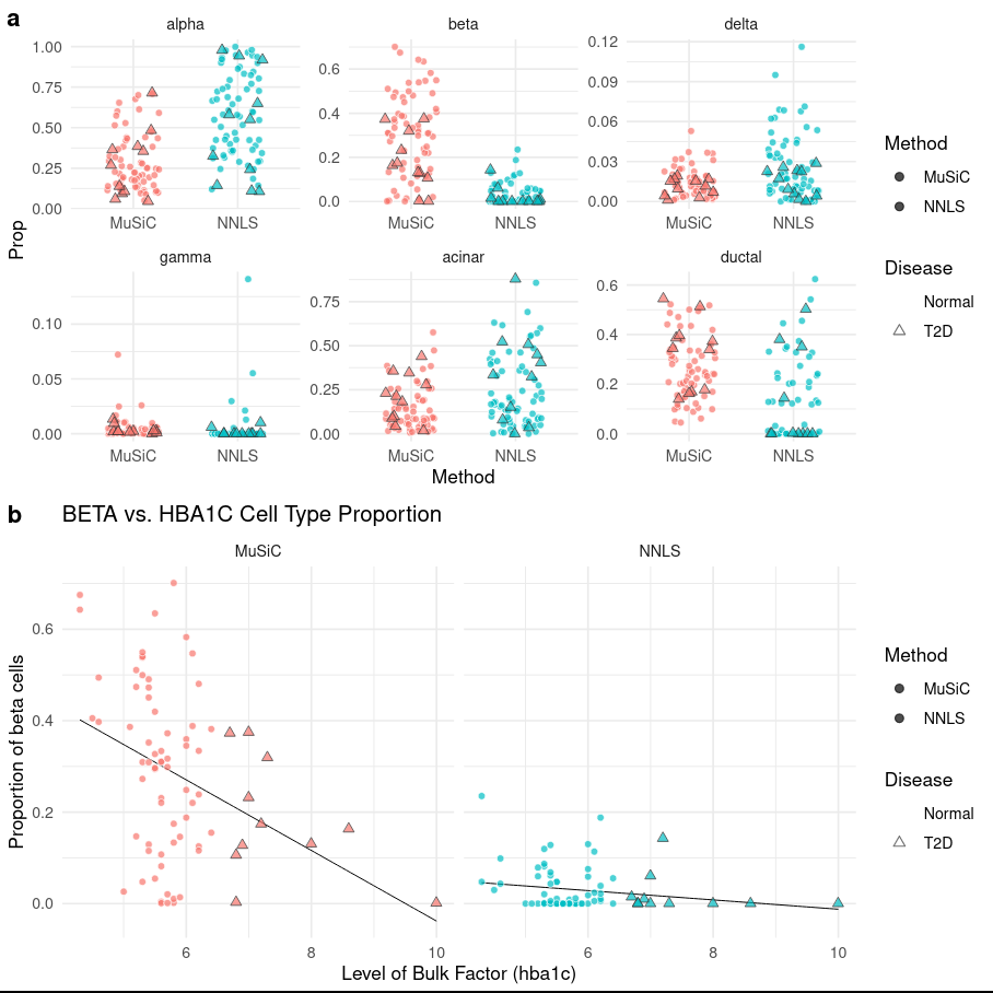 Open image in new tab
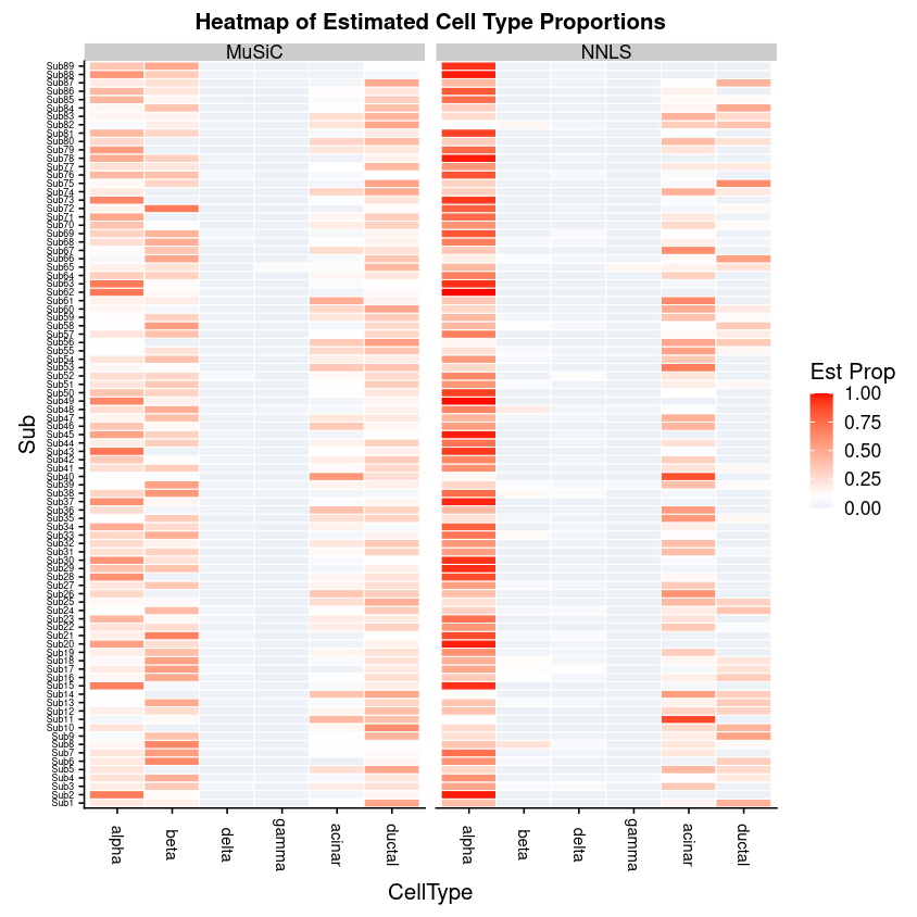 Open image in new tab
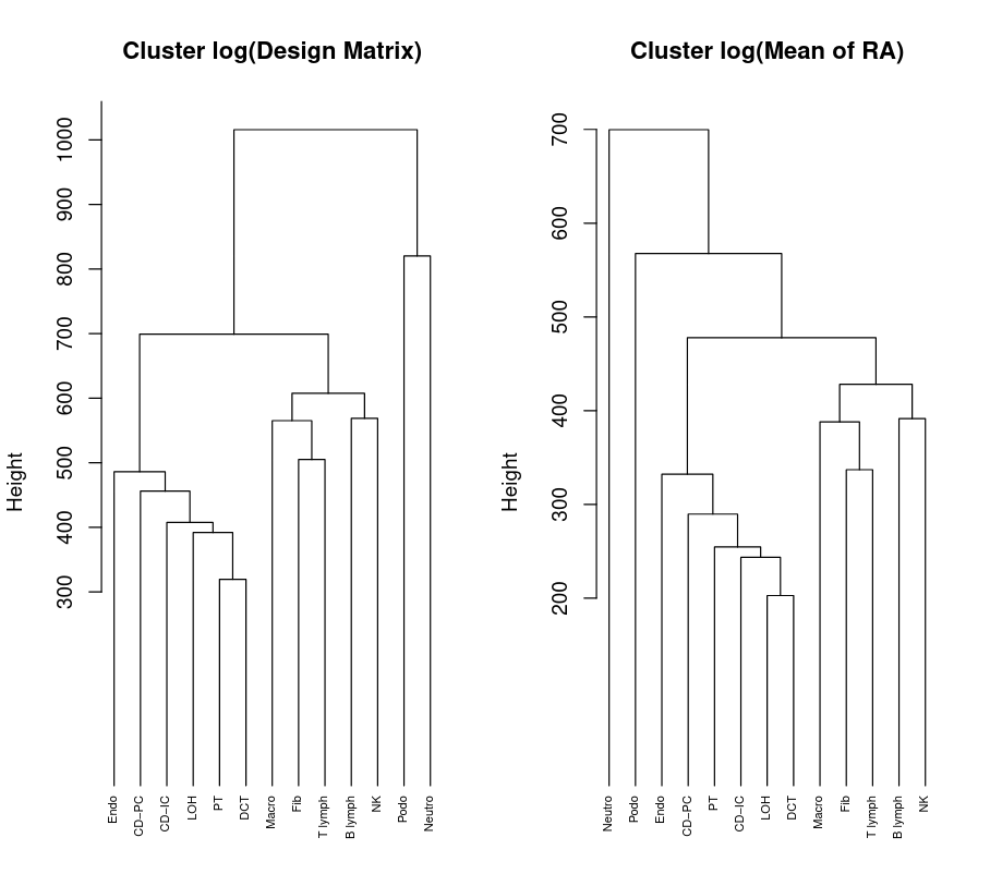 Open image in new tab
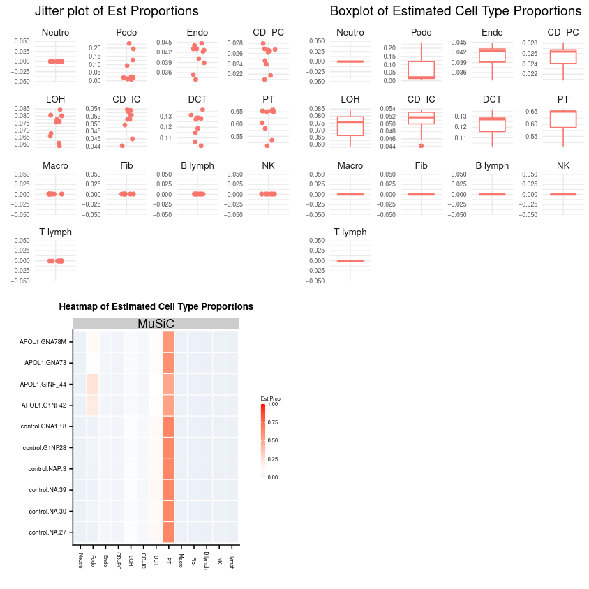 Open image in new tab
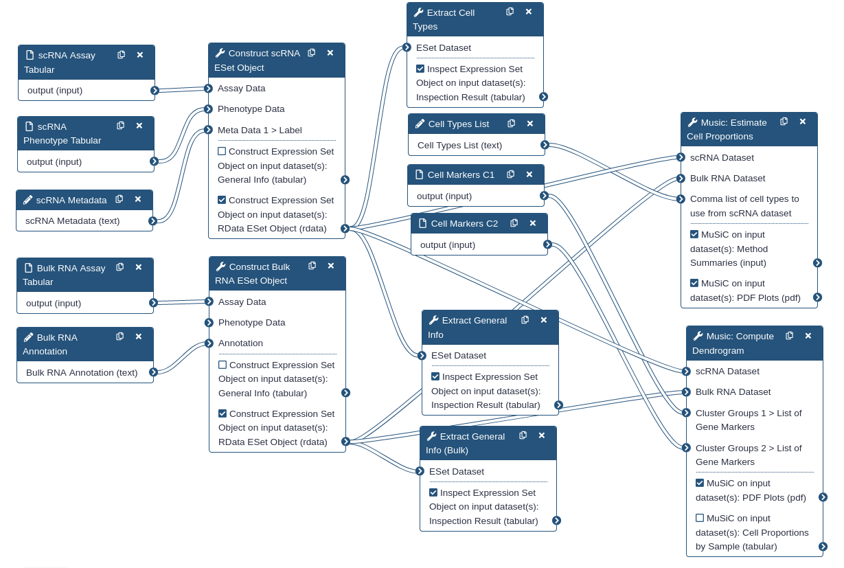 Open image in new tab
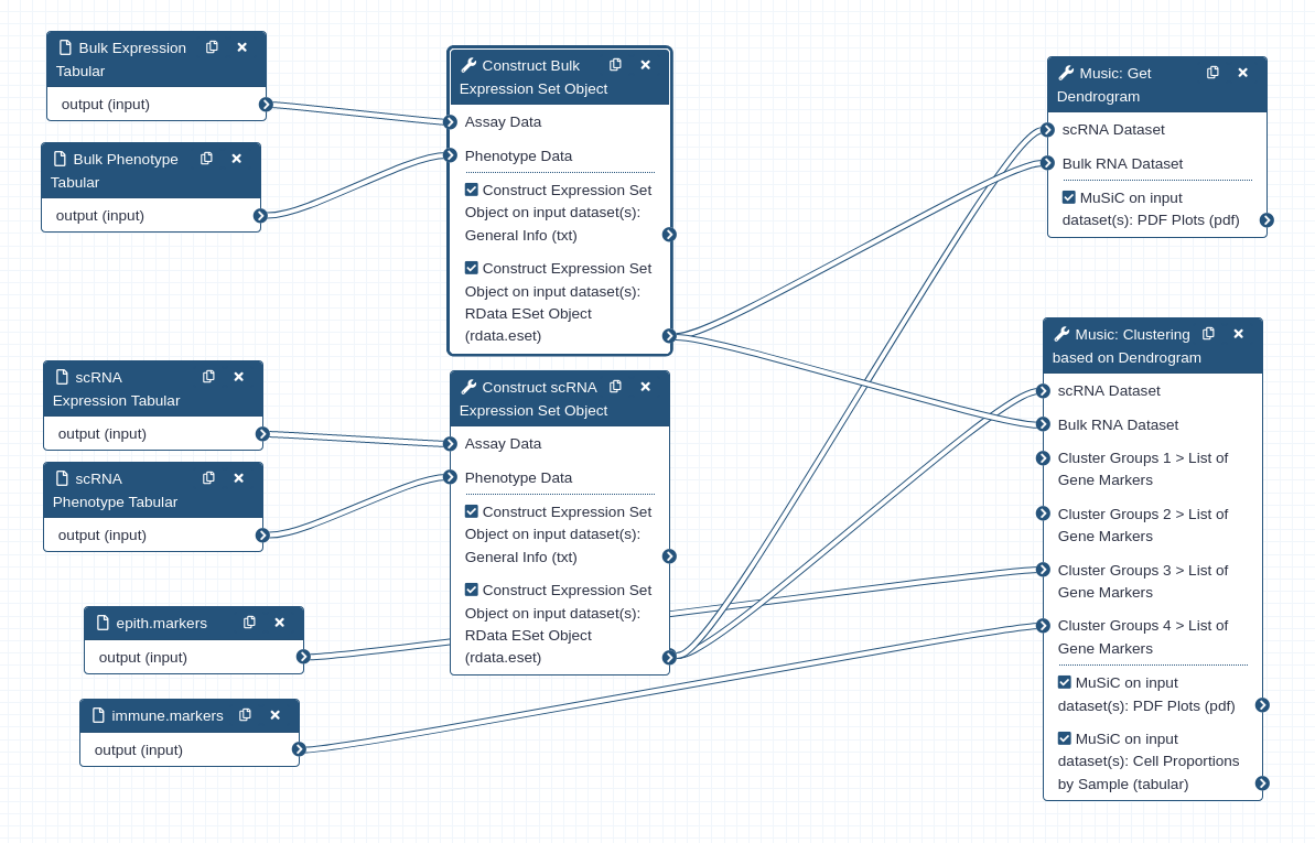 Open image in new tab