Similar to bulk ATAC-Seq, single-cell ATAC-Seq (scATAC-seq) leverages the hyperactive Tn5 Transposase to profile open chromatin regions but at single-cell resolution. Thus helps in understanding cell type-specific chromatin accessibility from a heterogeneous cell population.
Era of 10x Genomics
10x genomics has provided not only a cost-effective high-throughput solution to understanding sample heterogeneity at the individual cell level but has defined the standards of the field that many downstream analysis packages are now scrambling to accommodate. The gain in resolution reduces the granularity and noise issues that plagued the field of single-cell omics not long ago, where now individual clusters are much easier to decipher due to the added stability added by this gain in information.
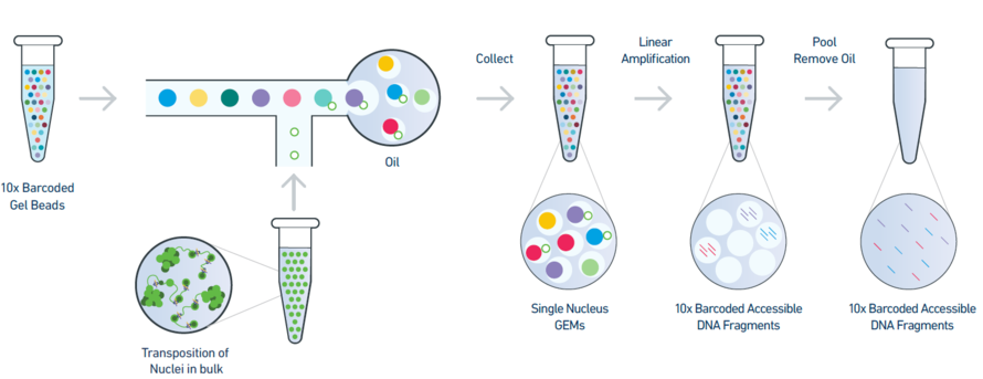
Figure 1: An overview of the 10x single-nuclei ATAC-seq library preparation
The 10X barcoded gel beads consist of a pool of barcodes which are used to separately index each cell. The individual gel barcodes are delivered to each cell via flow cytometry, where each cell is fed single-file along a liquid tube and tagged with a 10X gel bead. The cells are then isolated from one another within thousands of nanoliter droplets, where each droplet is described by a unique 10x barcode that all reads in that droplet are associated with. The oil is then removed and all (now barcoded) DNA reads are pooled together to be sequenced.
There are two main reagent kits used during the library preparation. Below we can see the layout of the primers used in both chemistries. We can ignore most of these as they are not relevant, namely: the P5 and P7 Illumina primers are used in the Illumina bridge amplification process; the Sample Index is an 8bp primer which is related to the Chromium system that balances nucleotide bias and ensures that there is no sample overlap during the multiplexed sequencing. The primer of interest to us is the Cell Barcode (CB). Unlike scRNA-seq, Unique Molecular Identifiers (UMIs) are not used in scATAC-seq.
There are two major chemistries (v1 and v2) used in 10x scATAC-seq library construction. Technically, v2 chemistry is more sensitive and has better data yield. But the final sequencing library is the same. Hence, same the data analysis applies to both chemistries. Both chemistries generate the 4 FASTQ files containing:
8bp sample index sequence (I1)
50bp forward read (R1)
16bp barcode sequence (R2)
49bp reverse read (R3)
The major differences to 10x scRNA-seq sequencing libraries are: (a) barcode sequences get a separate FASTQ file and (b) there are no UMIs. Note that as opposed to the traditional FASTQ naming, R3 contains reverse mate-pair and R2 contains barcode sequence.
The tutorial is structured into four parts. The first part deals with the preprocessing of FASTQ files, quality control and mapping. Then in the second part, we will identify the open chromatin regions. In the third part, we will create a count matrix using the cell barcode and open chromatin regions information. In the final part, we will filter out empty cells and less informative peaks to produce a high-quality count matrix.
Here we will use a published data set from 10x genomics consisting of thousand peripheral blood mononuclear cells (PBMCs) extracted from a healthy donor. Analyzing these full datasets requires several hours of computation time. Hence, we subsampled the data so that the tutorial can be finished in a reasonable amount of time with sensible results. In the sub-sampled data, we have the reads that were mostly generated from chromosome 21. The original data has FASTQ files from two sequencing lanes L001 and L002. We merged the sequences from both lanes. We also ignored the sample index FASTQ file as it is not useful for this analysis. Finally, we are left with three FASTQ files: R1 (forward reads), R2 (barcodes) and R3 (reverse reads).
atac_pbmc_1k_nextgem_S1_R1_001_chr21.fastq.gz
atac_pbmc_1k_nextgem_S1_R2_001_chr21.fastq.gz
atac_pbmc_1k_nextgem_S1_R3_001_chr21.fastq.gz
These files are provided in the Zenodo data repository. To analyze the full datasets, get the original FASTQ files from 10x genomics website
FASTQ processing and mapping
Data upload and organization
We import all three FASTQ files into a history.
Hands On: Data upload and organization
Create a new history and rename it (e.g. scATAC-seq 10X preprocessing tutorial)
To create a new history simply click the new-history icon at the top of the history panel:
Import the sub-sampled FASTQ data from Zenodo or from the data library (ask your instructor)
As an alternative to uploading the data from a URL or your computer, the files may also have been made available from a shared data library:
Go into Libraries (left panel)
Navigate to the correct folder as indicated by your instructor.
On most Galaxies tutorial data will be provided in a folder named GTN - Material –> Topic Name -> Tutorial Name.
Select the desired files
Click on Add to Historygalaxy-dropdown near the top and select as Datasets from the dropdown menu
In the pop-up window, choose
“Select history”: the history you want to import the data to (or create a new one)
Click galaxy-uploadUpload at the top of the activity panel
Select galaxy-wf-editPaste/Fetch Data
Paste the link(s) into the text field
Press Start
Close the window
Question
Inspect all the uploaded FASTQ files by clicking on the galaxy-eye symbol.
Which FASTQ file contains the barcode sequence?
What is the length of the barcode?
In this case, R2 contains the cell barcodes
16bp
Attach cell barcodes to FASTQ headers
First, we will attach the barcodes from the barcodes FASTQ file to the ids of forward and reverse reads that carry the association between reads and barcodes throughout the analysis. We will use this information to demultiplex the cells at the end while creating the count matrix. We will be left with only two FASTQ files of forward and reverse reads after this step.
Comment
Sinto barcode ( Galaxy version 0.9.0+galaxy1) consumes the barcode sequence from the atac_pbmc_1k_nextgem_S1_R2_001_chr21.fastq.gz file and uses : delimiter to prepend it to both the forward and reverse read ids. The tool expects the same number of reads in all three FASTQ files and should be present in the same order.
Hands On
Sinto barcode ( Galaxy version 0.9.0+galaxy1) with the following parameters:
“Number of bases to extract from barcode-containing FASTQ”: 16
Comment: Sinto barcode output
After a successful run, the barcode sequences from the barcode FASTQ file are prepended to the read names. We can inspect the output FASTQ files by clicking on the galaxy-eye symbol of the barcoded read 1 file.
Now let’s proceed with the next steps QC, mapping and peak calling as we do with the bulk ATAC-Seq data. For a thorough description of bulk ATAC-Seq analysis, please follow the bulk ATAC-Seq data analysis tutorial. Here we use a slightly different workflow. Here we map reads using BWA-MEM instead of Bowtie2, then create ATAC fragments file that also stores the cell barcode information and finally use MACS2 for peak calling. Note that the workflow from bulk ATAC-seq tutorial should also result in similar set of peaks.
FASTQ Quality control
First things first. Let’s do a basic FASTQ quality control using FastQC
Hands On
FastQC ( Galaxy version 0.73+galaxy0) with the following parameters:
“Raw read data from your current history”: Use param-filesMultiple datasets to choose both barcoded read 1 and barcoded read 2 (outputs of Sinto barcodetool).
Inspect the web page output of FastQCtool for the barcoded read 1 sample.
Question
How many reads are in the FASTQ?
Which sections have a warning?
There are 685686 reads.
The 2 steps below have warnings:
Per base sequence content
It is well known that the Tn5 has a strong sequence bias at the insertion site. You can read more about it in Green et al. 2012.
Sequence Duplication Levels
The read library quite often has PCR duplicates that are introduced
simply by the PCR itself. We will remove these duplicates later on.
There is only a little amount of Nextera Transposase Sequence in the reads (see Adapter Content section of FastQC output). In this case, we skip the adapter trimming step and proceed to the mapping step. If your data has a significant amount of Nextera Transposase Sequences, then proceed to adapter trimming using either cutadapt or Trim Galore!. Trim Galore can automatically detect the adapter sequence. If you use Cutadapt, follow the bulk ATAC-Seq tutorial Trimming Reads step.
Mapping reads to a reference genome
Now we map the reads to a reference genome using BWA-MEM ( Galaxy version 0.7.17.2).
Hands On: Mapping
Map with BWA-MEM ( Galaxy version 0.7.17.2) with the following parameters:
“Using reference genome”: hg38
In “Single or Paired-end reads”: Paired
In “Select first set of reads “: barcoded read 1 (output of Sinto barcodetool)
In “Select second set of reads “: barcoded read 2 (output of Sinto barcodetool)
“Select analysis mode”: 1.Simple Illumina mode
“BAM sorting mode”: Sort by chromosomal coordinates
Peak calling
In scRNA-seq we always have the standard set of genes (usually downloaded from public databases) to quantify the expression levels. For scATAC-seq, there are no such reference open chromatin regions because the regions of chromatin accessibility are tissue dependent. Hence, we first have to detect open chromatin regions. There are several ways of doing this. The most common ways are the following:
Find a published bulk ATAC-seq data that is the closest to your scATAC-seq data and use the regions from the bulk ATAC-seq data
Chunk the genome into equal-sized bins and use these bins as reference locations for quantification
Combine the data from all the cells of the scATAC-seq data together and detect open chromatin regions from the data. Later use these detected regions for quantification
In this tutorial, we opt for the 3rd option.
Create scATAC-seq fragments file
An ATAC-seq fragment file is a BED file with Tn5 integration sites, the cell barcode associated with the fragment, and the frequency of the sequenced fragment. PCR duplicates are collapsed. Here we filter out the alignments with low mapping quality.
Comment: on Tn5 insertion
When Tn5 cuts an accessible chromatin locus it inserts adapters separated by 9bp (Kia et al. 2017):
This means, to have the read start site reflecting the center of where Tn5 bound, the reads on the positive strand should be shifted 4 bp to the right and reads on the negative strands should be shifted 5 bp to the left as in Buenrostro et al. 2013. Genrich can apply these shifts when ATAC-seq mode is selected. In most cases, we do not have 9bp resolution so we don’t take it into account but if you are interested in the footprint, this is important.
Hands On: Create scATAC fragments
Sinto fragments ( Galaxy version 0.9.0+galaxy1) with the following parameters:
“Input BAM file”: mapped reads in BAM format (output of Map with BWA-MEMtool)`
“Minimum MAPQ required to retain fragment”: 30
“Regular expression used to extract cell barcode from read name”: [^:]* (matches all characters up to the first colon)
“Number of bases to shift Tn5 insertion position by on the forward strand”: 4
“Number of bases to shift Tn5 insertion position by on the reverse strand”: -5
“Take cell barcode into account when collapsing duplicate fragments”: Yes
bedtools SortBED ( Galaxy version 2.30.0+galaxy2) with the following parameters:
“Sort the following BED/bedGraph/GFF/VCF/EncodePeak file *“: fragments BED (output of Sinto fragmentstool)`
“Sort by”: chromosome, then by start position (asc)
Rename the dataset sorted fragments
Call Peaks
We have now finished the data preprocessing. Next, to find regions corresponding to potential open chromatin regions, we want to identify regions where reads have piled up (peaks) greater than the background read coverage. The tools which are currently used are Genrich and MACS2. MACS2 is more widely used.
At this step, two approaches exist:
The first one is to select only pairs whose fragment length is below 100bp corresponding to nucleosome-free regions and to use a peak calling like you would do for a ChIP-seq, joining signal between mates. The disadvantage of this approach is that you can only use it if you have paired-end data and you will miss small open regions where only one Tn5 is bound.
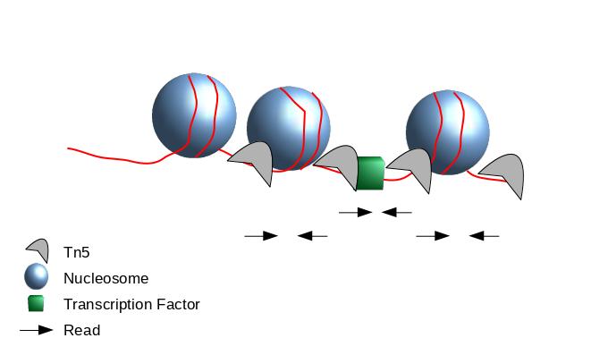
The second one chosen here is to use all reads to be more exhaustive. In this approach, it is very important to re-center the signal of each read on the 5’ extremity (read start site) as this is where Tn5 cuts. Indeed, you want your peaks around the nucleosomes and not directly on the nucleosome:
Figure 4: Scheme of ATAC-Seq reads relative to nucleosomes
If we only assess the coverage of the 5’ extremity of the reads, the data would be too sparse and it would be impossible to call peaks. Thus, we will extend the start sites of the reads by 200bp (100bp in each direction) to assess coverage. We call peaks with MACS2. In order to get the coverage centered on the 5’ extended 100bp on each side we will use --shift -100 and --extend 200:
MACS2 callpeak ( Galaxy version 2.1.1.20160309.6) with the following parameters:
“Are you pooling Treatment Files?”: No
“ChIP-Seq Treatment File”: sorted fragments
“Do you have a Control File?”: No
“Format of Input Files”: Single-end BED
“Effective genome size”: H. sapiens (2.7e9)
“Build Model”: Do not build the shifting model (--nomodel)
“Set extension size”: 200
“Set shift size”: -100. It needs to be - half the extension size to be centered on the 5’.
“Additional Outputs”:
Check Peaks as tabular file (compatible with MultiQC)
Check Peak summits
Check Scores in bedGraph files
In “Advanced Options”:
“Composite broad regions”: No broad regions
“Use a more sophisticated signal processing approach to find subpeak summits in each enriched peak region”: Yes
“How many duplicate tags at the exact same location are allowed?”: all
Comment: Why keeping all duplicates is important
We previously removed duplicates using Sinto fragmenttool using paired-end information. If two pairs had identical R1 but different R2, we knew it was not a PCR duplicate. Because we converted the BAM to BED we lost the pair information. If we keep the default (removing duplicates) one of the 2 identical R1 would be filtered out as duplicate.
Comment: BED / encode narrowPeak format
If you are not familiar with BED format or encode narrowPeak format, see the BED Format
Count matrix creation
Now we have ATAC fragments with cell barcode information as well as the peaks to create a scATAC count matrix. In the context of ATAC-seq, the peaks are also often called features. But the term feature is a generic term that denotes a peak in the case of scATAC-seq data and a gene in case of scRNA-seq data. So the count matrix we build is similar to that of scRNA-seq data with the exception that here we have open chromatin regions instead of genes. In this tutorial, both the terms feature and peak indicate an open chromatin region.
For count matrix creation, we will use Build count matrix from EpiScanpy tool suite. It takes fragments file and the peaks in either BED format or directly a narrowPeak file of MACS2 output. Regardless of file type, the tool only considers the first 3 columns which contain chromosome id, start and end positions of the peak regions. Parameters like --call-summits from our MACS2 run can result in different peaks with the same peak boundaries. It is always a good practice to remove duplicate peak regions so that our final count matrix will have unique features.
Hands On: Extract unique peak regions
Unique occurrences of each record ( Galaxy version 1.1.0) with the following parameters:
“File to scan for unique values”: narrow Peaks (output of MACS2tool)
In “Advanced Options”: Show Advanced Options
“Column start”: Column: 1
“Column end”: Column: 3
Question
How many peak regions were duplicated?
There were initially 1229 regions in the narrow Peaks file. Now there are 1046 regions after deduplication. Around 15% (184) of regions have the same peak boundaries.
AnnData
The most common format, called AnnData, stores the matrix as well as gene and cell annotations in a concise, compressed and extremely readable manner:
Figure 6:AnnData format stores a count matrix X together with annotations of observations (i.e. cells) obs, variables (i.e. peaks) var and unstructured annotations uns.
This format is used by Scanpy (Wolf et al. 2018) and EpiScanpy (Danese et al. 2021) tool suites for analyzing single-cell omics data. So we need first to import the matrix and annotations of peaks and cells (present in fragments BED file) into an AnnData object.
Hands On: Build count matrix with EpiScanpy
Build count matrix with EpiScanpy ( Galaxy version 0.3.2+galaxy1) with the following parameters:
“ATAC fragments file”: sorted fragments
“Features file”: output of Unique tool tool
“Normalize peak sizes?”: Keep the peaks as they are
In “Select the chromosomes of the species you are considering”: Custom list of chromosomes
“Enter comma seperated list of chromosome ids (without chr prefix)”: 21
Rename the generated file to PBMC 1k chr21 Anndata
Check that the format is h5ad
In this example data, our reads are from the chr21. Hence, we input 21 for chromosome ids. For human or mouse genomes, directly select from the dropdown list. Make sure that all the canonical chromosomes are present in the fragments file.
Because the AnnData format is an extension of the HDF5 format, i.e. a binary format, an AnnData object can not be inspected directly in Galaxy by clicking on the galaxy-eye (View data) icon. Instead, we need to use a dedicated tool from the AnnData suite.
Hands On: Inspect an AnnData object
Inspect AnnData ( Galaxy version 0.7.5+galaxy1) with the following parameters:
param-file“Annotated data matrix”: PBMC 1k chr21 Anndata
“What to inspect?”: General information about the object
Inspect the generated file
Question
AnnData object with n_obs × n_vars = 27388 × 1046
How many observations are there? What do they represent?
How many variables are there? What do they represent?
There are 27,388 observations, representing the cells.
There are 1046 variables, representing the peaks.
Comment: Faster Method for General Information
To view general information of any Anndata file:
Click on the name of the dataset in the history to expand it.
General Anndata information would be given in the expanded box:
e.g.
[n_obs x n_vars]
-    27388 x 1046
For more specific queries, Inspect AnnData ( Galaxy version 0.7.5+galaxy1) is required.
Inspect AnnData ( Galaxy version 0.7.5+galaxy1) with the following parameters:
param-file“Annotated data matrix”: PBMC 1k chr21 Anndata
The file is a table with 27,388 lines (observations or cells) and 1046 columns (variables or peaks): the count matrix for each of the 1046 peaks and 27,388 cells. The 1st row contains the peak location as an annotation of the columns and the 1st column the barcodes of the cells as an annotation of the rows.
Inspect AnnData ( Galaxy version 0.7.5+galaxy1) with the following parameters:
param-file“Annotated data matrix”: PBMC 1k chr21 Anndata
“What to inspect?”: Key-indexed observations annotation (obs)
The file is tabular with annotations of the observations. i.e. the cells. Here there are only the barcodes as annotation, so only one column, being also the index for the count matrix.
Inspect AnnData ( Galaxy version 0.7.5+galaxy1) with the following parameters:
param-file“Annotated data matrix”: PBMC 1k chr21 Anndata
“What to inspect?”: Key-indexed annotation of variables/features (var)
The file is tabular with annotations of the variables, i.e. the peaks.
Producing a Quality Count Matrix
We just created a count matrix with all detected peaks and non-empty barcodes. In this section of the tutorial, we will filter the features and barcodes by a series of quality assessments to generate a high-quality count matrix. The final count matrix can be used for further downstream analysis like clustering, differential chromatin analysis and cell type annotation.
The current matrix contains peaks from chromosome 21 only and is too small to carry out this type of analysis. From this step onwards we will use the full count matrix generated from the original FASTQ files. Please import the following anndata file to start:
What do you observe in comparison to a scRNA-seq count matrix?
There are 441038 barcodes and 70120 features
The initial number of barcodes in this raw count matrix is in the same range as the scRNA-seq data. But there is roughly double the number of features compared to a scRNA-seq dataset. The number of features varies from dataset to dataset. Based on the tools and parameters used for peak calling, the size of the initial feature set can grow up to several hundred of thousands.
Initial filtering to remove potential empty features and cells
First remove any potential empty features or barcodes. A non-empty cell should have a minimum number of non-empty features and a non-empty feature should be present in a minimum number of non-empty cells. Here we will different minimum thresholds for filtering cells and features.
Hands On: Initial filtering
scATAC-seq Preprocessing with EpiScanpy ( Galaxy version 0.3.2+galaxy1) with the following parameters:
“Annotated data matrix”: atac_pbmc_1k_uniq_peaks.h5ad
“Method used for filtering”: Filter cell outliers based on counts and numbers of features expressed, using 'pp.filter_cells'
“Filter”: Minimum number of features expressed
“Minimum features”: 100
scATAC-seq Preprocessing with EpiScanpy ( Galaxy version 0.3.2+galaxy1) with the following parameters:
“Annotated data matrix”: Output of the previous (pp.filter_cells) step
“Method used for filtering”: Filter features based on counts and numbers of features expressed, using 'pp.filter_features'
“Filter”: Minimum number of cells expressed
“Minimum features”: 1
Question
How much data was filtered out?
The resulting matrix has dimensions of 1815 x 67766, i.e., more than 99.5% of the cells and less than 4% of features were filtered out. This indicates the high sparsity of the count matrix.
Quality control and visualization
We will first plot the number of features per cell. This information is stored as nb_features layer of observations. As we are dealing with numbers with huge variances, it is sometimes hard to visualize them. Hence, we compute the log of nb_features first then plot the absolute and log values together.
Hands On: Violing plots of number of features
scATAC-seq Preprocessing with EpiScanpy ( Galaxy version 0.3.2+galaxy1) with the following parameters:
“Annotated data matrix”“: Output of previous (pp.filter_features) step
“Method used for filtering”: Compute log10 of nb_features
Check if observations have an extra log_nb_features in addition to nb_features layer.
Rename the resulting dataset to PBMC 1k after initial filtering
Plot with scanpy ( Galaxy version 1.7.1+galaxy0) with the following parameters:
param-file“Annotated data matrix”: PBMC 1k after initial filtering
“Method used for plotting”: Generic: Violin plot, using 'pl.violin'
“Keys for accessing variables”: Subset of variables in 'adata.var_names' or fields of '.obs'
“Keys for accessing variables”: nb_features, log_nb_features
In “Violin plot attributes”:
“Add a stripplot on top of the violin plot”: Yes
“Add a jitter to the stripplot”: Yes
“Size of the jitter points”: 0.4
“Display keys in multiple panels”: Yes
In “Parameters for seaborn.violinplot”:
“Color for all of the elements”: DarkCyan
Question
What trends of the data do you observe in the plots?
Figure 7: Violin plot of number of features per cell after initial filtering
Both plots indicate that there are two distinct sets of cells:
Cells with an acceptable number of open chromatin regions.
Cells with only a few detected peaks. These cells are uninformative and should be excluded.
To determine decent filtering thresholds, we will further look at some histograms of cell-peak coverage trends. We will plot histograms of the number of open features per cell and feature commonness in cells.
Hands On: Coverage cells
scATAC-seq Preprocessing with EpiScanpy ( Galaxy version 0.3.2+galaxy1) with the following parameters:
“Annotated data matrix”“: PBMC 1k after initial filtering
“Method used for filtering”: Coverage cells: Histogram of the number of open features (in the case of ATAC-seq data) per cell, using 'pp.coverage_cells'
“Binarized matrix?”: No
“Minimum number of cells or minimum number of features to be indicated in the plot”: 1000
scATAC-seq Preprocessing with EpiScanpy ( Galaxy version 0.3.2+galaxy1) with the following parameters:
“Annotated data matrix”“: PBMC 1k after initial filtering
“Method used for filtering”: Coverage cells: Histogram of the number of open features (in the case of ATAC-seq data) per cell, using 'pp.coverage_cells'
“Binarized matrix?”: No
“Log transform?”: Yes
“Minimum number of cells or minimum number of features to be indicated in the plot”: 1000
Now observe the plots
Question
What information do you see in these plots?
Do you think our minimum number of features threshold of 1000 indicated in the plot makes sense?
Figure 8: Histogram of the number of open chromatin regions per cellOpen image in new tab
Figure 9: Histogram of the number of open chromatin regions per cell in log scale
The plots show the number of open chromatin regions per cell in 50 bins on the x-axis and the number of cells per bin on the y-axis. It is basically a histogram of the number of open chromatin regions per cell.
From the first plot with absolute counts, we see that with our threshold of 1000, we can separate between the cells with few detected peaks and cells with high chromatin accessibility.
Hands On: Coverage features
scATAC-seq Preprocessing with EpiScanpy ( Galaxy version 0.3.2+galaxy1) with the following parameters:
“Annotated data matrix”“: PBMC 1k after initial filtering
“Method used for filtering”: Coverage features: Distribution of the feature commonness in cells, using 'pp.coverage_features'
“Binarized matrix?”: No
“Minimum number of cells or minimum number of features to be indicated in the plot”: 5
scATAC-seq Preprocessing with EpiScanpy ( Galaxy version 0.3.2+galaxy1) with the following parameters:
“Annotated data matrix”“: PBMC 1k after initial filtering
“Method used for filtering”: Coverage features: Distribution of the feature commonness in cells, using 'pp.coverage_features'
“Binarized matrix?”: No
“Log transform?”: Yes
“Minimum number of cells or minimum number of features to be indicated in the plot”: 5
Now observe the plots
Question
What information do you see in these plots?
Do you think our minimum number of cells threshold of 5 indicated in the plot makes sense?
Figure 11: Histogram of feature commonness in cells in log scale
The plots show a histogram of the number of cells sharing a feature. As we initially pooled the data from all the cells to detect the peaks, it is expected to see only a small number of cells have more than 10000 peaks in common.
The red vertical line of our 5 cells threshold is nearly at the left end of the histogram representing the majority of the features have at least 5 cells in common.
From the log scale plot it is also clear that there is a sharp increase in the feature commonness from at least 10 cells (x-axis 1.0).
So our threshold of 5 is a decent cutoff for filtering out the features. From the plots, only a very few non-informative features are left to be filtered out.
Final filtering to acquire quality cells and features
Based on the above QC plots, we will filter out all the cells with less than 1000 features and all the features that have less than 5 cells in common. Additionally, we will also filter out extreme outlier cells (which can be seen in the initial violin plot or coverage cells plot) with more than 12500 features.
Hands On: Final filtering based on QC plots
scATAC-seq Preprocessing with EpiScanpy ( Galaxy version 0.3.2+galaxy1) with the following parameters:
“Annotated data matrix”: PBMC 1k after initial filtering
“Method used for filtering”: Filter cell outliers based on counts and numbers of features expressed, using 'pp.filter_cells'
“Filter”: Minimum number of features expressed
“Minimum features”: 1000
scATAC-seq Preprocessing with EpiScanpy ( Galaxy version 0.3.2+galaxy1) with the following parameters:
“Annotated data matrix”: Output of previous (pp.filter_cells) step
“Method used for filtering”: Filter cell outliers based on counts and numbers of features expressed, using 'pp.filter_cells'
“Filter”: Maximum number of features expressed
“Minimum features”: 12500
scATAC-seq Preprocessing with EpiScanpy ( Galaxy version 0.3.2+galaxy1) with the following parameters:
“Annotated data matrix”: Output of previous (pp.filter_cells) step
“Method used for filtering”: Filter features based on counts and numbers of features expressed, using 'pp.filter_features'
“Filter”: Minimum number of cells expressed
“Minimum features”: 5
Question
What are the dimensions of the count matrix after the final filtering?
The resulting matrix has 1024 cells and 67719 peaks. The number of cells after filtering is close to what we expect in this dataset.
Conclusion
In this tutorial, we have learned how to map reads from 10X ATAC-seq data, identify open chromatin regions from aggregated cell data and generate a count matrix in Anndata format. We also performed quality control and filtered out empty and uninformative cells and features to generate a high-quality count matrix for downstream analysis.
Further information, including links to documentation and original publications, regarding the tools, analysis techniques and the interpretation of results described in this tutorial can be found here.
References
Green, B., C. Bouchier, C. Fairhead, N. L. Craig, and B. P. Cormack, 2012 Insertion site preference of Mu, Tn5, and Tn7 transposons. Mobile DNA 3: 3. 10.1186/1759-8753-3-3
Kia, A., C. Gloeckner, T. Osothprarop, N. Gormley, E. Bomati et al., 2017 Improved genome sequencing using an engineered transposase. BMC Biotechnology 17: 10.1186/s12896-016-0326-1
Danese, A., M. L. Richter, K. Chaichoompu, D. S. Fischer, F. J. Theis et al., 2021 EpiScanpy: integrated single-cell epigenomic analysis. Nature Communications 12: 5228. https://www.nature.com/articles/s41467-021-25131-3
Feedback
Did you use this material as an instructor? Feel free to give us feedback on how it went.
Did you use this material as a learner or student? Click the form below to leave feedback.
Hiltemann, Saskia, Rasche, Helena et al., 2023 Galaxy Training: A Powerful Framework for Teaching! PLOS Computational Biology 10.1371/journal.pcbi.1010752
Batut et al., 2018 Community-Driven Data Analysis Training for Biology Cell Systems 10.1016/j.cels.2018.05.012
@misc{single-cell-scatac-preprocessing-tenx,
author = "Pavankumar Videm",
	title = "Pre-processing of 10X Single-Cell ATAC-seq Datasets (Galaxy Training Materials)",
	year = "",
	month = "",
	day = "",
	url = "\url{https://training.galaxyproject.org/training-material/topics/single-cell/tutorials/scatac-preprocessing-tenx/tutorial.html}",
	note = "[Online; accessed TODAY]"
}
@article{Hiltemann_2023,
	doi = {10.1371/journal.pcbi.1010752},
	url = {https://doi.org/10.1371%2Fjournal.pcbi.1010752},
	year = 2023,
	month = {jan},
	publisher = {Public Library of Science ({PLoS})},
	volume = {19},
	number = {1},
	pages = {e1010752},
	author = {Saskia Hiltemann and Helena Rasche and Simon Gladman and Hans-Rudolf Hotz and Delphine Larivi{\`{e}}re and Daniel Blankenberg and Pratik D. Jagtap and Thomas Wollmann and Anthony Bretaudeau and Nadia Gou{\'{e}} and Timothy J. Griffin and Coline Royaux and Yvan Le Bras and Subina Mehta and Anna Syme and Frederik Coppens and Bert Droesbeke and Nicola Soranzo and Wendi Bacon and Fotis Psomopoulos and Crist{\'{o}}bal Gallardo-Alba and John Davis and Melanie Christine Föll and Matthias Fahrner and Maria A. Doyle and Beatriz Serrano-Solano and Anne Claire Fouilloux and Peter van Heusden and Wolfgang Maier and Dave Clements and Florian Heyl and Björn Grüning and B{\'{e}}r{\'{e}}nice Batut and},
	editor = {Francis Ouellette},
	title = {Galaxy Training: A powerful framework for teaching!},
	journal = {PLoS Comput Biol}
}
Congratulations on successfully completing this tutorial!
Do you want to extend your knowledge?
Follow one of our recommended follow-up trainings:
Questions:
 Open image in new tab
 Open image in new tab

Open image in new tab
 Open image in new tab
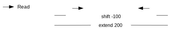 Open image in new tab
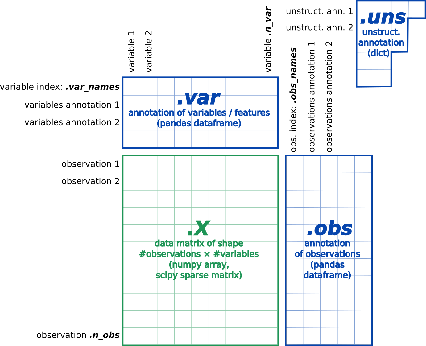 Open image in new tab
Open image in new tab
Open image in new tab
Open image in new tab
Open image in new tab
Open image in new tab
