Single-cell Assay for Transposase-Accessible Chromatin using sequencing (scATAC-seq) analysis is a method to decipher the chromatin states of the analyzed cells. In general, genes are only expressed in accessible (i.e. “open”) chromatin and not in closed chromatin.
By analyzing which genomic sites have an open chromatin state, cell-type specific patterns of gene accessibility can be determined.
scATAC-seq is particularly useful for analyzing tissue containing different cell populations, such as peripheral blood mononuclear cells (PBMCs).
In this tutorial we will analyze scATAC-seq data using the tool suites SnapATAC2 (Zhang et al. 2024) and Scanpy (Wolf et al. 2018).
With both of these tool suites we will perform preprocessing, clustering and identification of scATAC-seq datasets from 10x Genomics.
The analysis will be performed using a dataset of PBMCs containing ~4,620 single nuclei.
Did you know we have a unique Single Cell Omics Lab with all our single cell tools highlighted to make it easier to use on Galaxy? We recommend this site for all your single cell analysis needs, particularly for newer users.
The Single Cell Omics Lab is a different view of the underlying Galaxy server that organises tools and resources better for single-cell users! It also provides a platform for communities to engage and connect; distribute more targeted news and events; and highlight community-specific funding sources.
Tools are frequently updated to new versions. Your Galaxy may have multiple versions of the same tool available. By default, you will be shown the latest version of the tool. This may NOT be the same tool used in the tutorial you are accessing. Furthermore, if you use a newer tool in one step, and try using an older tool in the next step… this may fail! To ensure you use the same tool versions of a given tutorial, use the Tutorial mode feature.
Open your Galaxy server
Click on the curriculum icon on the top menu, this will open the GTN inside Galaxy.
Navigate to your tutorial
Tool names in tutorials will be blue buttons that open the correct tool for you
Note: this does not work for all tutorials (yet)
You can click anywhere in the grey-ed out area outside of the tutorial box to return back to the Galaxy analytical interface
Warning: Not all browsers work!
We’ve had some issues with Tutorial mode on Safari for Mac users.
Try a different browser if you aren’t seeing the button.
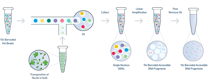
ATAC-seq utilizes a hyperactive Tn5 transposase (Kia et al. 2017) to ligate adaptors to genome fragments, created by the transposase. Performing ATAC-seq on individual cells used to be an expensive and time-consuming labour.
The 10X Chromium NextGEM system made scATAC-seq a cost-effective method for gaining high-resolution data with a simple protocol.
After the transposition of nuclei in bulk, individual nuclei are put into Gel beads in Emulsion (GEM), containing unique 10x cell barcodes and sequencing adaptors for Illumina sequencing.
Figure 1: An overview of the 10X single-nuclei ATAC-seq library preparation
Data
The 5k PBMCs dataset for this tutorial is available for free from 10X Genomics. The blood samples were collected from a healthy donor and were prepared following the Chromium Next GEM scATAC-seq protocol. After sequencing on Illumina NovaSeq, the reads were processed by the Cell Ranger ATAC 2.0.0 pipeline from 10X to generate a Fragments File.
The Fragments File is a tabular file in a BED-like format, containing information about the position of the fragments on the chromosome and their corresponding 10x cell barcodes.
SnapATAC2 requires 3 input files for the standard pathway of processing:
fragments_file.tsv: A tabular file containing the chromosome positions of the fragments and their corresponding 10x cell barcodes.
chrom_sizes.txt: A tabular file of the number of bases of each chromosome of the reference genome
gene_annotation.gtf.gz: A tabular file listing genomic features of the reference genome (GENCODE GRCh38)
A chromosome sizes file can be generated using the tool Compute sequence length ( Galaxy version 1.0.3).
The reference genome can either be selected from cached genomes or uploaded to the galaxy history.
Comment
This tutorial starts with a fragment file.
SnapATAC2 also accepts mapped reads in a BAM file.
SnapATAC2 Preprocessing ( Galaxy version 2.6.4+galaxy1) with the following parameters:
“Method used for preprocessing”: Convert a BAM file to a fragment file, using 'pp.make_fragment_file'
param-file“File name of the BAM file”: BAM_500-PBMC (Input dataset)
param-toggle“Indicate whether the BAM file contain paired-end reads”: Yes
“How to extract barcodes from BAM records?”: From read names using regular expressions
“Extract barcodes from read names of BAM records using regular expressions”: (................):
Comment
Not every regular expression type is supported.
This expression selects 16 characters if they are followed by a colon. Only the cell barcodes of the BAM file will match.
Rename the generated file to Fragments 500 PBMC
Now you can continue with either the fragments_file from earlier or the new file Fragments 500 PBMC.
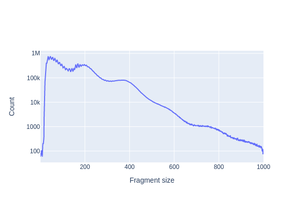
galaxy-info The tool pp.make_fragment_filetool has implemented additional quality control (QC) measures. These filter out larger fragments, which will be noticeable in the log-scale fragment size distribution.
galaxy-info Please note that Fragments 500 PBMC only contains 500 PBMCs and thus the clustering will produce different outputs compared to the outputs generated by fragments_file (with 5k PBMC).
Preprocessing
Preprocessing of the scATAC-seq data contained in the fragment file with SnapATAC2 begins with importing the files and computing basic QC metrics.
SnapATAC2 compresses and stores the fragments into an AnnData object.
AnnData
The AnnData format was initially developed for the Scanpy package and is now a widely accepted data format to
store annotated data matrices in a space-efficient manner.
Import files to SnapATAC2
Hands On: Create an AnnData object
SnapATAC2 Preprocessing ( Galaxy version 2.6.4+galaxy1) with the following parameters:
“Method used for preprocessing”: Import data fragment files and compute basic QC metrics, using 'pp.import_data'
param-file“Fragment file, optionally compressed with gzip or zstd”: fragments_file.tsv (Input dataset)
param-toggle“Whether the fragment file has been sorted by cell barcodes”: No
This tool requires the fragment file to be sorted according to cell barcodes.
If pp.make_fragment_filetool was used to generate the fragment file, this has automatically been done.
Otherwise, the setting “sorted by cell barcodes” should remain No.
Rename the generated file to Anndata 5k PBMC
Check that the format is h5ad
Because the AnnData format is an extension of the HDF5 format, i.e. a binary format, an AnnData object can not be inspected directly in Galaxy by clicking on the galaxy-eye (View data) icon.
Instead, we need to use a dedicated tool from the AnnData suite.
Hands On: Inspect an AnnData object
Inspect AnnData ( Galaxy version 0.10.3+galaxy0) with the following parameters:
param-file“Annotated data matrix”: Anndata 5k PBMC
“What to inspect?”: General information about the object
How many observations are there? What do they represent?
How many variables are there?
There are 14232 observations, representing the cells.
There are 0 variables, representing genomic regions. This is because genome-wide 500-bp bins are only added after initial filtering.
Many toolsets producing outputs in AnnData formats in Galaxy, provide the general information by default:
Click on the name of the dataset in the history to expand it.
General Anndata information will be given in the expanded box:
e.g.
[n_obs x n_vars]
-    14232 × 0
details This feature isn’t the most reliable and might display:
[n_obs x n_vars]
-    1 × 1
In such cases and for more specific queries, Inspect AnnData ( Galaxy version 0.10.3+galaxy0) is required.
Calculate and visualize QC metrics
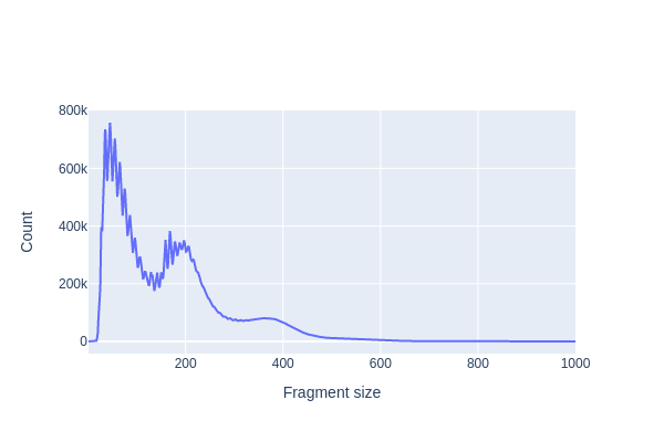
Hands On: Fragment-size distribution
SnapATAC2 Plotting ( Galaxy version 2.6.4+galaxy1) with the following parameters:
“Method used for plotting”: Plot fragment size distribution, using 'pl.frag_size_distr'
param-file“Annotated data matrix”: Anndata 5k PBMC (output of pp.import_datatool)
galaxy-eye Inspect the .png output
SnapATAC2 Plotting ( Galaxy version 2.6.4+galaxy1) with the following parameters:
“Method used for plotting”: Plot fragment size distribution, using 'pl.frag_size_distr'
param-file“Annotated data matrix”: Anndata 5k PBMC (output of pp.import_datatool)
“Change the y-axis (fragment counts) to log scale”: Yes
galaxy-eye Inspect the .png output
Question
What distinct features do the plots have? And what do they represent?
Which fragments are generally from open chromatin?
3 peaks are clearly visible (at <100-bp, ~200-bp and ~400-bp). The smallest fragments are from nucleosome-free regions, while the larger peaks of 200- and 400-bp contain mono- and di-nucleosome fragments, respectively.
The small fragments (<100-bp) are from open chromatin reads, since the Tn5 transposase could easily access the loosely packed DNA (Yan et al. 2020).
The transcription start site enrichment (TSSe) is another important QC metric. Nucleosome-free fragments are expected to be enriched at transcription start sites (TSS). TSSe shows increased fragmentation of chromatin around the TSS. This suggests open and accessible nucleosome-free chromatin.
TSSe is used as a QC metric, since an increased enrichment around TSS regions suggests that the experiment has captured biological meaningful genomic features.
TSSe scores of individual cells can be calculated using SnapATAC2’s metrics.tsse function.
Hands On: Calculate and Plot TSSe
SnapATAC2 Preprocessing ( Galaxy version 2.6.4+galaxy1) with the following parameters:
“Method used for preprocessing”: Compute the TSS enrichment score (TSSe) for each cell, using 'metrics.tsse'
param-file“Annotated data matrix”: Anndata 5k PBMC (output of pp.import_datatool)
param-file“GTF/GFF file containing the gene annotation”: gene_annotation.gtf.gz (Input dataset)
Rename the generated file to Anndata 5k PBMC TSSe or add the tag galaxy-tagsTSSe to the dataset:
Datasets can be tagged. This simplifies the tracking of datasets across the Galaxy interface. Tags can contain any combination of letters or numbers but cannot contain spaces.
To tag a dataset:
Click on the dataset to expand it
Click on Add Tagsgalaxy-tags
Add tag text. Tags starting with # will be automatically propagated to the outputs of tools using this dataset (see below).
Press Enter
Check that the tag appears below the dataset name
Tags beginning with # are special!
They are called Name tags. The unique feature of these tags is that they propagate: if a dataset is labelled with a name tag, all derivatives (children) of this dataset will automatically inherit this tag (see below). The figure below explains why this is so useful. Consider the following analysis (numbers in parenthesis correspond to dataset numbers in the figure below):
a set of forward and reverse reads (datasets 1 and 2) is mapped against a reference using Bowtie2 generating dataset 3;
dataset 3 is used to calculate read coverage using BedTools Genome Coverageseparately for + and - strands. This generates two datasets (4 and 5 for plus and minus, respectively);
datasets 4 and 5 are used as inputs to Macs2 broadCall datasets generating datasets 6 and 8;
datasets 6 and 8 are intersected with coordinates of genes (dataset 9) using BedTools Intersect generating datasets 10 and 11.
Now consider that this analysis is done without name tags. This is shown on the left side of the figure. It is hard to trace which datasets contain “plus” data versus “minus” data. For example, does dataset 10 contain “plus” data or “minus” data? Probably “minus” but are you sure? In the case of a small history like the one shown here, it is possible to trace this manually but as the size of a history grows it will become very challenging.
The right side of the figure shows exactly the same analysis, but using name tags. When the analysis was conducted datasets 4 and 5 were tagged with #plus and #minus, respectively. When they were used as inputs to Macs2 resulting datasets 6 and 8 automatically inherited them and so on… As a result it is straightforward to trace both branches (plus and minus) of this analysis.
SnapATAC2 Plotting ( Galaxy version 2.6.4+galaxy1) with the following parameters:
“Method used for plotting”: Plot the TSS enrichment vs. number of fragments density figure, using 'pl.tsse'
param-file“Annotated data matrix”: Anndata 5k PBMC TSSe (output of metrics.tssetool)
galaxy-eye Inspect the .png output
High-quality cells can be identified in the plot of TSSe scores against a number of unique fragments for each cell.
Question
Where are high-quality cells located in the plot?
Based on this plot, how should the filter be set?
The cells in the upper right are high-quality cells, enriched for TSS. Fragments in the lower left represent low-quality cells or empty droplets and should be filtered out.
Setting the minimum number of counts at 5,000 and the minimum TSS enrichment to 10.0 is an adequate filter.
Filtering
Based on the TSSe plot the cells can be filtered by TSSe and fragment counts.
Hands On: Filter cells
SnapATAC2 Preprocessing ( Galaxy version 2.6.4+galaxy1) with the following parameters:
“Method used for preprocessing”: Filter cell outliers based on counts and numbers of genes expressed, using 'pp.filter_cells'
param-file“Annotated data matrix”: Anndata 5k PBMC TSSe (output of metrics.tssetool)
“Minimum number of counts required for a cell to pass filtering”: 5000
“Minimum TSS enrichemnt score required for a cell to pass filtering”: 10.0
“Maximum number of counts required for a cell to pass filtering”: 100000
Rename the generated file to Anndata 5k PBMC TSSe filtered or add the tag galaxy-tagsfiltered to the dataset
galaxy-eye Inspect the general information of the .h5ad output
How have the observations changed, compared to the first Anndata 5k PBMC AnnData file?
What does this tell us about the quality of the data?
There are only 4564 observations, compared to the initial 14232 observations.
And the obs: 'tsse' has been added (but already during metrics.tssetool)
The empty droplets and low-quality cells have been filtered out, leaving us with 4564 high-quality cells.
Feature selection
Currently, our AnnData matrix does not contain any variables. The variables will be added in the following step with the function pp.add_tile_matrix.
This creates a cell-by-bin matrix containing insertion counts across genome-wide 500-bp bins.
After creating the variables, the most accessible features are selected.
Hands On: Select features
SnapATAC2 Preprocessing ( Galaxy version 2.6.4+galaxy1) with the following parameters:
“Method used for preprocessing”: Generate cell by bin count matrix, using 'pp.add_tile_matrix'
param-file“Annotated data matrix”: Anndata 5k PBMC TSSe filtered (output of pp.filter_cellstool)
“The size of consecutive genomic regions used to record the counts”: 500
“The strategy to compute feature counts”: "insertion": based on the number of insertions that overlap with a region of interest
SnapATAC2 Preprocessing ( Galaxy version 2.6.4+galaxy1) with the following parameters:
“Method used for preprocessing”: Perform feature selection, using 'pp.select_features'
param-file“Annotated data matrix”: Anndata tile_matrix (output of pp.add_tile_matrixtool)
“Number of features to keep”: 250000
Comment: Select features
Including more features improves resolution and can reveal finer details, but it may also introduce noise.
To optimize results, experiment with the n_features parameter to find the most appropriate value for your dataset.
To demonstrate the differences when selecting features, the following UMAP plots are the outputs from processing with a number of features between 1,000 and 500,000.
Fewer features result in fewer, but larger clusters. Selecting a lot of features will output more granular clusters and the compute time will increase.
How did n_vars change compared to Anndata 5k PBMC TSSe filtered
Where are the selected features stored in the count matrix?
There are 6,062,095 variables, compared to 0 in TSSe filtered.
Selected features are stored in var: 'selected'.
Doublet removal
Doublets are removed by calling a customized scrublet (Wolock et al. 2019) algorithm. pp.scrublet will identify potential doublets and the function pp.filter_doublets removes them.
During single-cell sequencing, multiple nuclei can be encapsulated into the same 10x gel bead. The resulting multiplets (>97% of which are doublets) produce sequences from both cells.
Doublets can confound the results by appearing as “new” clusters or artifactual intermediary cell states.
These problematic doublets are called neotypic doublets, since they appear as “new” cell types.
Scrublet (Single-cell Remover of Doublets) is an algorithm which can detect neotypic doublets that produce false results.
The algorithm first simulates doublets by combining random pairs of observed cell features.
The observed features of the “cells” are then compared to the simulated doublets and scored on their doublet probability.
SnapATAC2’s pp.filter_doublets then removes all cells with a doublet probability >50%.
Cell doublets were removed. n_obs was reduced from 4564 to 4430 cells.
The outputs of pp.scrublet are stored in observations obs: 'doublet_probability', 'doublet_score' and in unstructured annotations uns: 'scrublet_sim_doublet_score'. The output of pp.filter_doublets is stored in uns: 'doublet_rate'.
Dimension reduction
Dimension reduction is a very important step during the analysis of single cell data. During this, the complex multi-dimensional data is projected into lower-dimensional space, while the lower-dimensional embedding of the complex data retains as much information as possible. Dimension reduction enables batch correction, data visualization and quicker downstream analysis since the data is more simplified and the memory usage is reduced (Zhang et al. 2024).
Dimension reduction algorithms can be either linear or non-linear.
Linear methods are generally computationally efficient and well scalable.
A popular linear dimension reduction algorithm is:
PCA (Principle Component Analysis), implemented in Scanpy (please check out our Scanpy tutorial for an explanation).
Nonlinear methods however are well suited for multimodal and complex datasets.
in contrast to linear methods, which often preserve global structures, non-linear methods have a locality-preserving character.
This makes non-linear methods relatively insensitive to outliers and noise while emphasizing natural clusters in the data (Belkin and Niyogi 2003)
As such, they are implemented in many algorithms to visualize the data in 2 dimensions (f.ex. UMAP embedding).
The nonlinear dimension reduction algorithm, through matrix-free spectral embedding, used in SnapATAC2 is a very fast and memory efficient non-linear algorithm (Zhang et al. 2024).
Spectral embedding utilizes an iterative algorithm to calculate the spectrum (eigenvalues and eigenvectors) of a matrix without computing the matrix itself.
The outputs of tl.spectral are stored in unstructured annotations uns: 'spectral_eigenvalue' and as multidimensional observations obsm: 'X_spectral'.
UMAP embedding
With the already reduced dimensionality of the data stored in X_spectral, the cells can be further embedded (i.e. transformed into lower dimensions) with Uniform Manifold Approximation and Projection (UMAP).
UMAP projects the cells and their relationship to each other into 2-dimensional space, which can be easily visualized (McInnes et al. 2018).
Hands On: UMAP embedding
SnapATAC2 Clustering ( Galaxy version 2.6.4+galaxy1) with the following parameters:
“Dimension reduction and Clustering”: Compute Umap, using 'tl.umap'
param-file“Annotated data matrix”: Anndata 5k PBMC spectral (output of tl.spectraltool)
“Use the indicated representation in ‘.obsm’“: X_spectral
Rename the generated file to Anndata 5k PBMC UMAP or add the tag galaxy-tagsUMAP to the dataset
Clustering
During clustering, cells that share similar accessibility profiles are organized into clusters. SnapATAC2 utilizes graph-based community clustering with the Leiden algorithm (Traag et al. 2019).
This method takes the k-nearest neighbor (KNN) graph as input data and produces well-connected communities.
Community clustering
Hands On: Clustering analysis
SnapATAC2 Clustering ( Galaxy version 2.6.4+galaxy1) with the following parameters:
“Dimension reduction and Clustering”: Compute a neighborhood graph of observations, using 'pp.knn'
param-file“Annotated data matrix”: Anndata 5k PBMC UMAP (output of tl.umaptool)
SnapATAC2 Clustering ( Galaxy version 2.6.4+galaxy1) with the following parameters:
“Dimension reduction and Clustering”: Cluster cells into subgroups, using 'tl.leiden'
param-file“Annotated data matrix”: Anndata knn (output of pp.knntool)
“Whether to use the Constant Potts Model (CPM) or modularity”: modularity
Comment: CPM or modularity
make sure you selected modularity
the clusters produced by CPM are not represented well in the UMAP projections
Rename the generated file to Anndata 5k PBMC leiden or add the tag galaxy-tagsleiden to the dataset
galaxy-eye Inspect the general information of the .h5ad output
Where are the leiden clusters stored in the AnnData?
The clusters are stored in obs: 'leiden'
Plotting of clusters
Now that we have produced UMAP embeddings of our cells and have organized the cells into leiden clusters, we can now visualize this information with pl.umap.
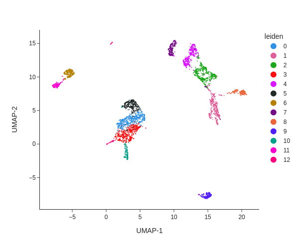
Hands On: Plotting the clusters
SnapATAC2 Plotting ( Galaxy version 2.6.4+galaxy1) with the following parameters:
“Method used for plotting”: Plot the UMAP embedding, using 'pl.umap'
param-file“Annotated data matrix”: Anndata 5k PBMC leiden (output of tl.leidentool)
“Color”: leiden
“Height of the plot”: 500
galaxy-eye Inspect the .png output
Question
How many leiden clusters were discovered?
What does the distance of clusters to each other tell us about their chromatin states?
There are 13 leiden clusters.
Clusters in close proximity (f.ex. clusters 0 and 5) share a similar chromatin accessibility profile (and very likely also a similar cell type), compared to a cluster further away (f.ex. cluster 9).
Cell cluster annotation
After clustering the cells, they must be annotated. This categorizes the clusters into known cell types. Manual Cell Annotation requires known marker genes and varying expression profiles of the marker genes among clusters.
Luckily, the marker genes for PBMCs are known (Sun et al. 2019).
Marker genes for other single cell datasets can also be found in databases such as PanglaoDB (Franzén et al. 2019). Using the known marker genes we can now annotate our clusters manually.
Gene matrix
Since our data currently doesn’t contain gene information, we have to create a cell-by-gene activity matrix using the function pp.make_gene_matrix.
Hands On: Task description
SnapATAC2 Preprocessing ( Galaxy version 2.6.4+galaxy1) with the following parameters:
“Method used for preprocessing”: Generate cell by gene activity matrix, using 'pp.make_gene_matrix'
param-file“Annotated data matrix”: Anndata 5k PBMC leiden (output of tl.leidentool)
param-file“GTF/GFF file containing the gene annotation”: gene_annotation.gtf.gz (Input dataset)
Rename the generated file to Anndata 5k PBMC gene_matrix or add the tag galaxy-tagsgene_matrix to the dataset
Please note that pp.make_gene_matrix removes all annotations except those stored in obs.
Therefore it might be necessary to remove propagating tags galaxy-tags (tags starting with #) from Anndata 5k PBMC gene_matrix.
Tags can be removed by expanding the dataset with a tag and clicking galaxy-cross next to the tag.
galaxy-eye Inspect the general information of the .h5ad output
What does n_vars represent in Anndata 5k PBMC gene_matrix and what did it represent in Anndata 5k PBMC leiden?
The variables now represent accessible genes. There are 60606 accessible genes in our samples. In Anndata 5k PBMC leiden and all earlier AnnData the variables represented the 6062095 fixed-sized genomic bins.
Imputation with Scanpy and MAGIC
Similar to scRNA-seq data, the cell-by-gene-activity matrix is very sparse. Additionally, high gene variance between cells, due to technical confounders, could impact the downstream analysis.
In scRNA-seq, filtering and normalization are therefore required to produce a high-quality gene matrix.
Since the cell-by-gene-activity matrix resembles the cell-by-gene-expression matrix of scRNA-seq, we can use the tools of the Scanpy (Wolf et al. 2018) tool suite to continue with our data.
The count matrices of single-cell data are sparse and noisy.
Confounding issues, such as “dropout” effects, where some mRNA or DNA-segments are not detected although they are present in the cell, also result in some cells missing important cell-type defining features.
These problems can obscure the data, as only the strongest gene-gene relationships are still detectable.
The Markov Affinity-based Graph Imputation of Cells (MAGIC) algorithm (van Dijk et al. 2018) tries to solve these issues by filling in missing data from some cells with transcript information from similar cells.
The algorithm calculates the likely gene expression of a single cell, based on similar cells and fills in the missing data to produce the expected expression.
MAGIC achieves this by building a graph from the data and using data diffusion to smooth out the noise.
How did n_vars change, compared to Anndata 5k PBMC gene_matrix?
Which data was ‘lost’, compared to Anndata 5k PBMC leiden, and must be added to the file in order to produce UMAP plots?
The number of genes was reduced from 60606 to 55106 by the filtering. Additional annotations were added, such as: obs: 'n_genes', 'n_counts', var: 'n_cells', 'n_counts' and uns: 'log1p'.
The UMAP embeddings obsm: 'X_umap' are missing and should be added to the Anndata in the next step. Without X_umap it won’t be possible to visualize the plots.
Copy-over embeddings
Hands On: Copy UMAP embedding
AnnData Operations ( Galaxy version 1.9.3+galaxy0) with the following parameters:
param-file“Input object in hdf5 AnnData format”: Anndata 5k PBMC magic (output of external.pp.magictool)
“Copy embeddings (such as UMAP, tSNE)”: Yes
“Keys from embeddings to copy”: X_umap
param-file“IAnnData objects with embeddings to copy”: Anndata 5k PBMC leiden
Comment: Annotations to copy
This tutorial only focuses on producing an UMAP plot with marker-genes.
If further analysis, with tools requiring more annotations, is intended, these can be added in a similar way as shown above.
f.ex. Peak and Motif Analysis with Snapatac2 peaks and motif ( Galaxy version 2.6.4+galaxy1) requires annotations from uns.
It is also possible to leave the input “Keys from embeddings to copy” empty, to copy all annotations of a given category such as obsm.
Rename the generated file to Anndata 5k PBMC magic UMAP or add the tag galaxy-tagsUMAP to the dataset
galaxy-eye Inspect the general information of the .h5ad output, to check if obsm contains X_umap
The gene activity of selected marker genes can now be visualized with Scanpy.
Hands On: Plot marker genes
Plot with Scanpy ( Galaxy version 1.9.6+galaxy3) with the following parameters:
param-file“Annotated data matrix”: output_h5ad (output of AnnData Operationstool)
“Method used for plotting”: Embeddings: Scatter plot in UMAP basis, using 'pl.umap'
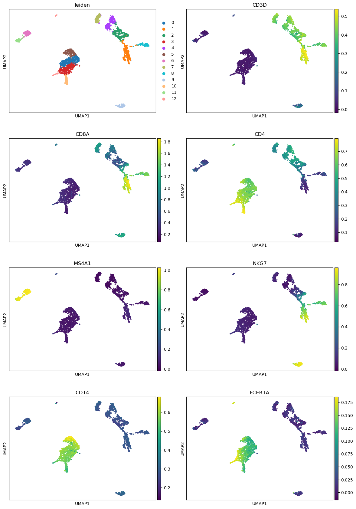
“Keys for annotations of observations/cells or variables/genes”: leiden, CD3D, CD8A, CD4, MS4A1, NKG7, CD14, FCER1A
param-toggle“Show edges?”: No
In “Plot attributes”
“Number of panels per row”: 2
Question
Are the marker genes selectively expressed in the clusters?
Which marker genes have overlapping expression profiles? And what could that imply?
Some marker genes, such as MS4A1 or CD8A, are only expressed in a few clusters (clusters 6+11 and clusters 1+8, respectively).
The marker gene CD3D is expressed in multiple clusters (1, 2, 4, 7 and 8). Overlapping expression profiles imply similar cell types since similar cell types have similar marker genes upregulated. In this case, CD3D expression classifies the cells in these clusters as T-cells.
Manual cluster annotation
Comparison of marker gene expression in our clusters with a table of canonical marker genes (Sun et al. 2019), enables us to annotate the clusters manually.
Cell type
Marker genes
CD8+ T cells
CD3D+, CD8A+, CD4-
CD4+ T cells
CD3D+, CD8A-, CD4+
B cells
CD3D-, MS4A1+
Natural killer (NK) cells
CD3D-, NKG7+
Monocytes
CD3D-, CD14+
Dendritic cells
CD3D-, FCER1A+
These canonical marker genes can match the clusters to known cell types:
Cluster
Cell type
0
Monocytes
1
CD8+ T cells
2
CD4+ T cells
3
Monocytes
4
CD4+ T cells
5
Monocytes
6
B cells
7
CD4+ T cells
8
CD8+ T cells
9
NK cells
10
Monocytes
11
B cells
12
Dendritic cells
Comment
Note that some clusters contain subtypes (f.ex. the annotated B cell clusters contain both naive and memory B cells). The cell-type annotation can be refined by choosing more specific marker genes.
To manually annotate the Leiden clusters, we will need to perform multiple steps:
Inspect the key-indexed observations of Anndata 5k PBMC gene_matrix magic UMAP
Cut the Leiden annotations out of the table
Upload a replace file containing the new cell type annotations for the Leiden clusters
Replace the values of the cluster annotation with cell type annotation
Add the cell type annotation to the AnnData
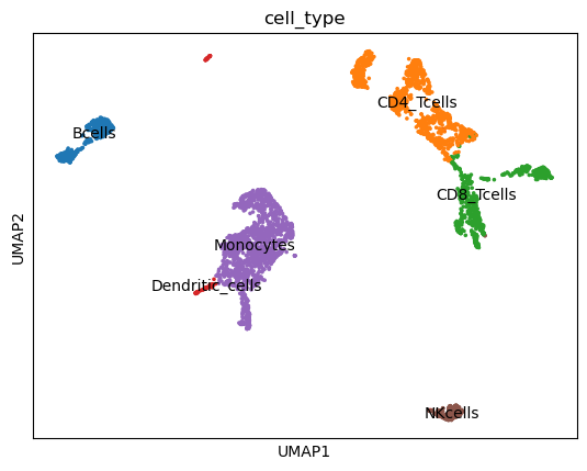
Plot the annotated cell types
Hands On: Manual annotation
Inspect AnnData ( Galaxy version 0.10.3+galaxy0) with the following parameters:
param-file“Annotated data matrix”: Anndata 5k PBMC gene_matrix magic UMAP
“What to inspect?”: Key-indexed observations annotation
Rename the generated file to 5k PBMC observations
galaxy-eye Inspect the generated file
Question
In which column is the Leiden annotation located?
The Leiden annotation is in column 8.
Column 1
Column 2
Column 3
Column 4
Column 5
Column 6
Column 7
Column 8
Column 9
Column 10
””
n_fragment
frac_dup
frac_mito
tsse
doublet_probability
doublet_score
leiden
n_genes
n_counts
AAACGAAAGACGTCAG-1
22070
0.5219425551271499
0.0
30.43315066436454
0.004634433324822066
0.009276437847866418
8
52303
16521.599844068267
AAACGAAAGATTGACA-1
10500
0.5345125681606597
0.0
29.10551296093465
0.004668403569267374
0.001088139281828074
1
54501
15020.42495602328
AAACGAAAGGGTCCCT-1
19201
0.5101785714285714
0.0
19.90011850347046
0.004634433324822066
0.009276437847866418
5
54212
16294.751533305309
AAACGAACAATTGTGC-1
13242
0.487399837417257
0.0
29.060913705583758
0.004660125753854076
0.0022172949002217295
7
53530
15456.629863655084
Cut columns ( Galaxy version 1.0.2) with the following parameters:
param-select“Cut columns”: c8
param-file“From”: 5k PBMC observations (output of Inspect AnnDatatool)
Yes. B-cells are far away from NK and T cells. Only the myeloid lineage of monocytes and dendritic cells are located close to each other. This might be due to the common progenitor cell lineage and thus a similar chromatin profile.
Yes. The most common cell types are T cells, followed by Monocytes and B cells. NK cells and Dendritic cells only make up a small percentage of PBMCs.
Conclusion
congratulations Well done, you’ve made it to the end! You might want to consult your results with this control history, or check out the full workflow for this tutorial.
In this tutorial, we produced a count matrix of scATAC-seq reads in the AnnData format and performed:
Preprocessing:
Plotting the fragment-size distributions
Calculating and plotting TSSe scores
Filtering cells and selecting features (fixed-size genomic bins)
Dimension reduction through Spectral embedding and UMAP
Clustering of cells via the Leiden method
Cluster annotation
Producing and filtering a cell by gene activity matrix
Data normalization and imputation with Scanpy and the MAGIC algorithm
Visualizing marker genes in the clusters
Manually annotating the cell types with selected marker genes
The scATAC-seq analysis can now continue with downstream analysis, for example differential peak analysis.
The SnapATAC2 tools for differential peak analysis are already accessible on Galaxy. However, there are no GTN trainings available yet. Until such a tutorial is uploaded, you can visit the SnapATAC2 documentation for a tutorial on differential peak analysis. And check out our example history and the exemplary workflow.
The tools are available in Galaxy under SnapATAC2 Peaks and Motif ( Galaxy version 2.6.4+galaxy1).
If you want to continue with differential peak analysis, please make sure that the AnnData object with the annotated cell types contains unspecified annotations for the reference sequences (uns: 'reference_sequences').
The section Copy-over embeddings explains how to copy annotations from one AnnData object to another.
You've Finished the Tutorial
Please also consider filling out the Feedback Form as well!
Key points
Single-cell ATAC-seq can identify open chromatin sites
Dimension reduction is required to simplify the data while preserving important information about the relationships of cells to each other.
Clusters of similar cells can be annotated to their respective cell-types
Frequently Asked Questions
Have questions about this tutorial? Have a look at the available FAQ pages and support channels
Further information, including links to documentation and original publications, regarding the tools, analysis techniques and the interpretation of results described in this tutorial can be found here.
References
Belkin, M., and P. Niyogi, 2003 Laplacian Eigenmaps for Dimensionality Reduction and Data Representation. Neural Computation 15: 1373–1396. 10.1162/089976603321780317
Kia, A., C. Gloeckner, T. Osothprarop, N. Gormley, E. Bomati et al., 2017 Improved genome sequencing using an engineered transposase. BMC Biotechnology 17: 10.1186/s12896-016-0326-1
Wolf, F. A., P. Angerer, and F. J. Theis, 2018 SCANPY: large-scale single-cell gene expression data analysis. Genome Biology 19: 10.1186/s13059-017-1382-0
Dijk, D. van, R. Sharma, J. Nainys, K. Yim, P. Kathail et al., 2018 Recovering Gene Interactions from Single-Cell Data Using Data Diffusion. Cell 174: 716–729.e27. 10.1016/j.cell.2018.05.061
Amemiya, H. M., A. Kundaje, and A. P. Boyle, 2019 The ENCODE Blacklist: Identification of Problematic Regions of the Genome. Scientific Reports 9: 10.1038/s41598-019-45839-z
Franzén, O., L.-M. Gan, and J. L. M. Björkegren, 2019 PanglaoDB: a web server for exploration of mouse and human single-cell RNA sequencing data. Database 2019: 10.1093/database/baz046
Sun, Z., L. Chen, H. Xin, Y. Jiang, Q. Huang et al., 2019 A Bayesian mixture model for clustering droplet-based single-cell transcriptomic data from population studies. Nature Communications 10: 10.1038/s41467-019-09639-3
Traag, V. A., L. Waltman, and N. J. van Eck, 2019 From Louvain to Leiden: guaranteeing well-connected communities. Scientific Reports 9: 10.1038/s41598-019-41695-z
Wolock, S. L., R. Lopez, and A. M. Klein, 2019 Scrublet: Computational Identification of Cell Doublets in Single-Cell Transcriptomic Data. Cell Systems 8: 281–291.e9. 10.1016/j.cels.2018.11.005
Yan, F., D. R. Powell, D. J. Curtis, and N. C. Wong, 2020 From reads to insight: a hitchhiker’s guide to ATAC-seq data analysis. Genome Biology 21: 10.1186/s13059-020-1929-3
Zhang, K., N. R. Zemke, E. J. Armand, and B. Ren, 2024 A fast, scalable and versatile tool for analysis of single-cell omics data. Nature Methods 21: 217–227. 10.1038/s41592-023-02139-9
Glossary
PBMCs
peripheral blood mononuclear cells
QC
quality control
TSS
transcription start sites
TSSe
transcription start site enrichment
UMAP
Uniform Manifold Approximation and Projection
scATAC-seq
Single-cell Assay for Transposase-Accessible Chromatin using sequencing
Feedback
Did you use this material as an instructor? Feel free to give us feedback on how it went.
Did you use this material as a learner or student? Click the form below to leave feedback.
Hiltemann, Saskia, Rasche, Helena et al., 2023 Galaxy Training: A Powerful Framework for Teaching! PLOS Computational Biology 10.1371/journal.pcbi.1010752
Batut et al., 2018 Community-Driven Data Analysis Training for Biology Cell Systems 10.1016/j.cels.2018.05.012
@misc{single-cell-scatac-standard-processing-snapatac2,
author = "Timon Schlegel",
	title = "Single-cell ATAC-seq standard processing with SnapATAC2 (Galaxy Training Materials)",
	year = "",
	month = "",
	day = "",
	url = "\url{https://training.galaxyproject.org/training-material/topics/single-cell/tutorials/scatac-standard-processing-snapatac2/tutorial.html}",
	note = "[Online; accessed TODAY]"
}
@article{Hiltemann_2023,
	doi = {10.1371/journal.pcbi.1010752},
	url = {https://doi.org/10.1371%2Fjournal.pcbi.1010752},
	year = 2023,
	month = {jan},
	publisher = {Public Library of Science ({PLoS})},
	volume = {19},
	number = {1},
	pages = {e1010752},
	author = {Saskia Hiltemann and Helena Rasche and Simon Gladman and Hans-Rudolf Hotz and Delphine Larivi{\`{e}}re and Daniel Blankenberg and Pratik D. Jagtap and Thomas Wollmann and Anthony Bretaudeau and Nadia Gou{\'{e}} and Timothy J. Griffin and Coline Royaux and Yvan Le Bras and Subina Mehta and Anna Syme and Frederik Coppens and Bert Droesbeke and Nicola Soranzo and Wendi Bacon and Fotis Psomopoulos and Crist{\'{o}}bal Gallardo-Alba and John Davis and Melanie Christine Föll and Matthias Fahrner and Maria A. Doyle and Beatriz Serrano-Solano and Anne Claire Fouilloux and Peter van Heusden and Wolfgang Maier and Dave Clements and Florian Heyl and Björn Grüning and B{\'{e}}r{\'{e}}nice Batut and},
	editor = {Francis Ouellette},
	title = {Galaxy Training: A powerful framework for teaching!},
	journal = {PLoS Comput Biol}
}
Funding
These individuals or organisations provided funding support for the development of this resource
Questions:
 Open image in new tab
 <code>obs</code>, variables (i.e. genes) <code>var</code> and unstructured annotations <code>uns</code>.")
High-quality cells can be identified in the plot of TSSe scores against a number of unique fragments for each cell.
Question
Open image in new tab
Open image in new tab
Open image in new tab