Metatranscriptomics analysis using microbiome RNA-seq data
| Author(s) |
|
| Editor(s) |
|
| Reviewers |
|
OverviewQuestions:
Objectives:
How to analyze metatranscriptomics data?
What information can be extracted of metatranscriptomics data?
How to assign taxa and function to the identified sequences?
Requirements:
Choose the best approach to analyze metatranscriptomics data
Understand the functional microbiome characterization using metatranscriptomic results
Understand where metatranscriptomics fits in ‘multi-omic’ analysis of microbiomes
Visualise a community structure
Time estimation: 5 hoursLevel: Introductory IntroductorySupporting Materials:Published: Nov 21, 2019Last modification: Jun 16, 2025License: Tutorial Content is licensed under Creative Commons Attribution 4.0 International License. The GTN Framework is licensed under MITpurl PURL: https://gxy.io/GTN:T00388rating Rating: 5.0 (2 recent ratings, 12 all time)version Revision: 6
In this tutorial we will perform a metatranscriptomics analysis based on the ASAIM workflow (Batut et al. 2018), using data from Kunath et al. 2018.
Comment: Two versions of this tutorialBecause this tutorial consists of many steps, we have made two versions of it, one long and one short.
This is the extended version. We will run every tool manually and discuss the results in detail. If you would like to run through the tutorial a bit quicker and use workflows to run groups of analysis steps (e.g. data cleaning) at once, please see the shorter version of this tutorial
You can also switch between the long and short version at the start of any section.
Introduction
Microbiomes play a critical role in host health, disease, and the environment. The study of microbiota and microbial communities has been facilitated by the evolution of technologies, specifically the sequencing techniques. We can now study the microbiome dynamics by investigating the DNA content (metagenomics), RNA expression (metatranscriptomics), protein expression (metaproteomics) or small molecules (metabolomics):
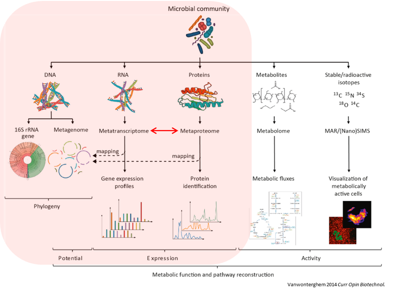
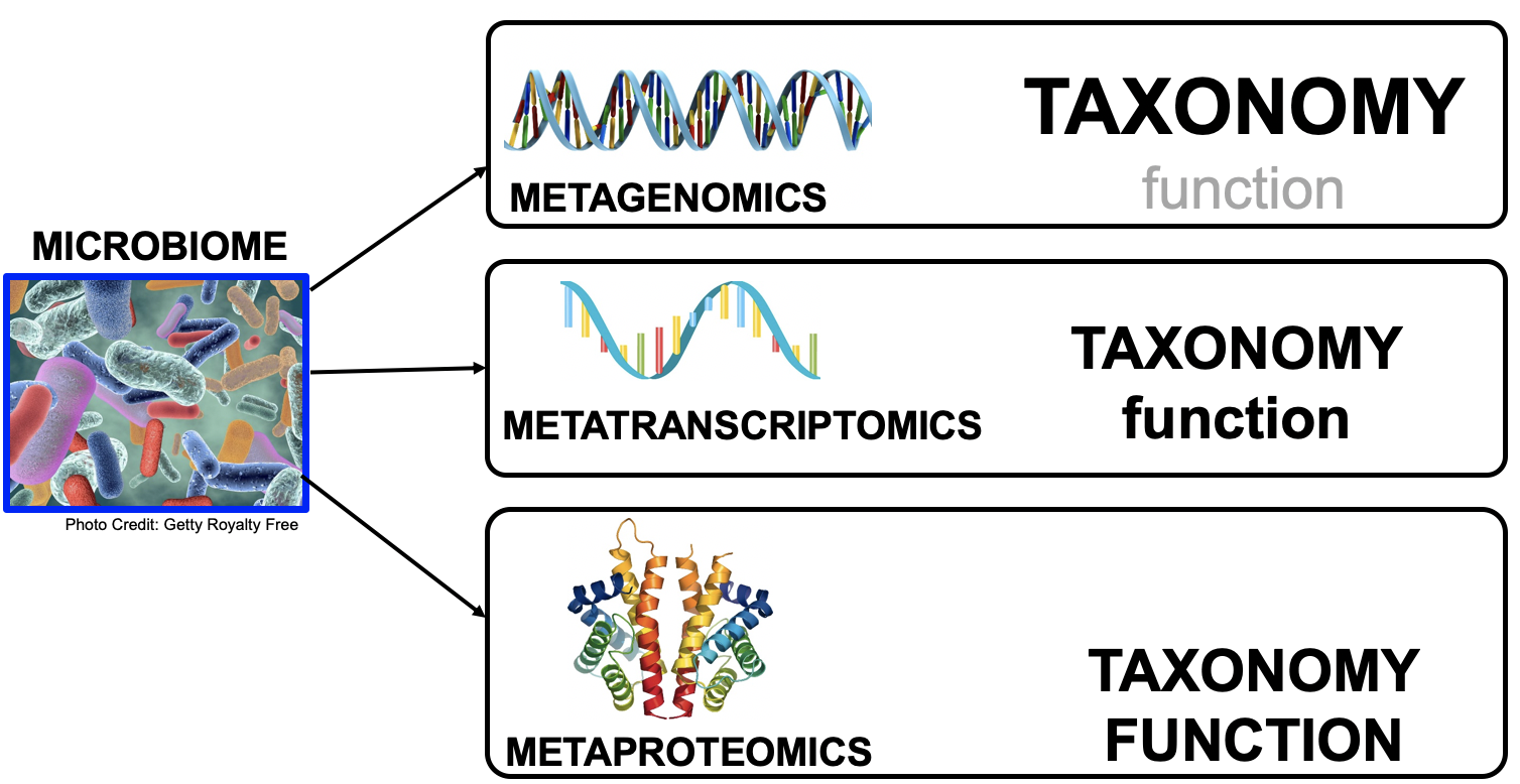
New generations of sequencing platforms coupled with numerous bioinformatic tools have led to a spectacular technological progress in metagenomics and metatranscriptomics to investigate complex microorganism communities. These techniques are giving insight into taxonomic profiles and genomic components of microbial communities. Metagenomics is packed with information about the present taxonomies in a microbiome, but do not tell much about important functions. That is where metatranscriptomics and metaproteomics play a big part.
In this tutorial, we will focus on metatranscriptomics.
Metatranscriptomics analysis enables understanding of how the microbiome responds to the environment by studying the functional analysis of genes expressed by the microbiome. It can also estimate the taxonomic composition of the microbial population. It provides scientists with the confirmation of predicted open‐reading frames (ORFs) and potential identification of novel sites of transcription and/or translation from microbial genomes. Furthermore, metatranscriptomics can enable more complete generation of protein sequences databases for metaproteomics.
To illustrate how to analyze metatranscriptomics data, we will use data from time-series analysis of a microbial community inside a bioreactor (Kunath et al. 2018). They generated metatranscriptomics data for 3 replicates over 7 time points. Before amplification the amount of rRNA was reduced by rRNA depletion. The sequencing libray was prepared with the TruSeq stranded RNA sample preparation, which included the production of a cDNA library.
In this tutorial, we focus on biological replicate A of the 1st time point. In a follow-up tutorial we will illustrate how to compare the results over the different time points and replicates. The input files used here are trimmed versions of the original files for the purpose of saving time and resources.
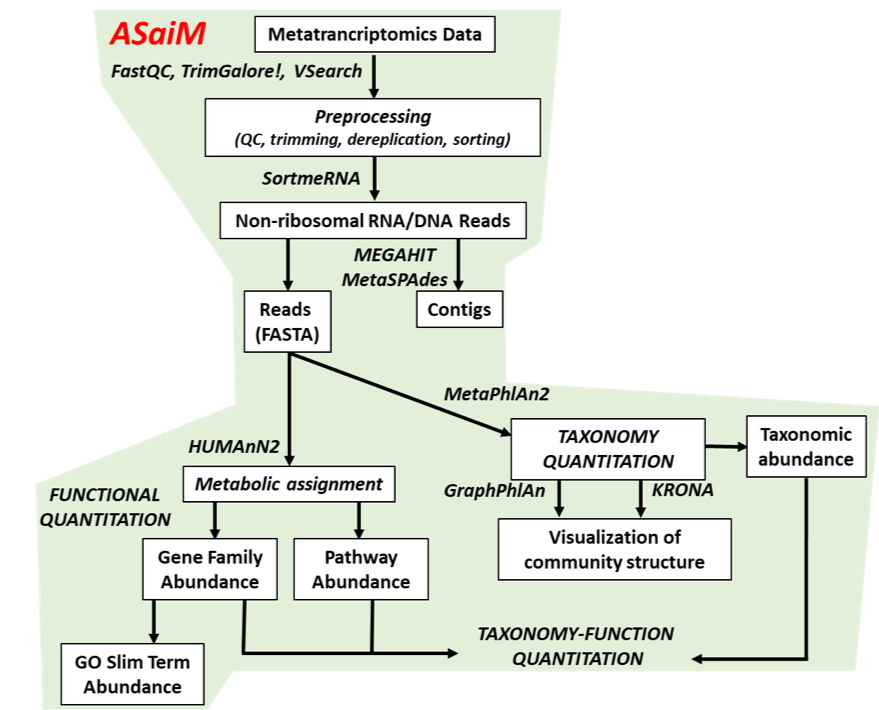
To analyze the data, we will follow the ASaiM workflow and explain it step by step. ASaiM (Batut et al. 2018) is an open-source Galaxy-based workflow that enables microbiome analyses. The workflow offers a streamlined Galaxy workflow for users to explore metagenomic/metatranscriptomic data in a reproducible and transparent environment. The ASaiM workflow has been updated by the GalaxyP team (University of Minnesota) to perform metatranscriptomics analysis of large microbial datasets (Mehta et al. 2021).
The workflow described in this tutorial takes in paired-end datasets of raw shotgun sequences (in FastQ format) as an input and proceeds to:
- Preprocess the reads
- Extract and analyze the community structure (taxonomic information)
- Extract and analyze the community functions (functional information)
- Combine taxonomic and functional information to offer insights into the taxonomic contribution to a function or functions expressed by a particular taxonomy.
A graphical representation of the ASaiM workflow which we will be using today is given below:
Comment: Workflow also applicable to metagenomics dataThe approach with the tools described here can also be applied to metagenomics data. What will change are the quality control profiles and the proportion of rRNA sequences.
AgendaIn this tutorial, we will cover:
Data upload
Hands On: Data upload
Create a new history for this tutorial and give it a proper name
To create a new history simply click the new-history icon at the top of the history panel:
- Click on galaxy-pencil (Edit) next to the history name (which by default is “Unnamed history”)
- Type the new name
- Click on Save
- To cancel renaming, click the galaxy-undo “Cancel” button
If you do not have the galaxy-pencil (Edit) next to the history name (which can be the case if you are using an older version of Galaxy) do the following:
- Click on Unnamed history (or the current name of the history) (Click to rename history) at the top of your history panel
- Type the new name
- Press Enter
Import
T1A_forwardandT1A_reversefrom Zenodo or from the data library (ask your instructor)https://zenodo.org/record/4776250/files/T1A_forward.fastqsanger https://zenodo.org/record/4776250/files/T1A_reverse.fastqsanger
- Copy the link location
Click galaxy-upload Upload at the top of the activity panel
- Select galaxy-wf-edit Paste/Fetch Data
Paste the link(s) into the text field
Press Start
- Close the window
As an alternative to uploading the data from a URL or your computer, the files may also have been made available from a shared data library:
- Go into Libraries (left panel)
- Navigate to the correct folder as indicated by your instructor.
- On most Galaxies tutorial data will be provided in a folder named GTN - Material –> Topic Name -> Tutorial Name.
- Select the desired files
- Click on Add to History galaxy-dropdown near the top and select as Datasets from the dropdown menu
In the pop-up window, choose
- “Select history”: the history you want to import the data to (or create a new one)
- Click on Import
As default, Galaxy takes the link as name, so rename them.
Rename galaxy-pencil the files to
T1A_forwardandT1A_reverse
- Click on the galaxy-pencil pencil icon for the dataset to edit its attributes
- In the central panel, change the Name field
- Click the Save button
Check that the datatype is
fastqsanger(e.g. notfastq). If it is not, please change the datatype tofastqsanger.
- Click on the galaxy-pencil pencil icon for the dataset to edit its attributes
- In the central panel, click galaxy-chart-select-data Datatypes tab on the top
- In the galaxy-chart-select-data Assign Datatype, select
fastqsangerfrom “New Type” dropdown
- Tip: you can start typing the datatype into the field to filter the dropdown menu
- Click the Save button


Preprocessing
exchange Switch to short tutorial
Quality control
During sequencing, errors are introduced, such as incorrect nucleotides being called. These are due to the technical limitations of each sequencing platform. Sequencing errors might bias the analysis and can lead to a misinterpretation of the data.
Sequence quality control is therefore an essential first step in your analysis. In this tutorial we use similar tools as described in the tutorial “Quality control”:
- FastQC generates a web report that will aid you in assessing the quality of your data
- MultiQC combines multiple FastQC reports into a single overview report
- Cutadapt for trimming and filtering
Hands On: Quality control
- FastQC ( Galaxy version 0.74+galaxy1) with the following parameters:
- param-files “Short read data from your current history”: both
T1A_forwardandT1A_reversedatasets selected with Multiple datasets
- Click on param-files Multiple datasets
- Select several files by keeping the Ctrl (or COMMAND) key pressed and clicking on the files of interest
Inspect the webpage output of FastQC tool for the
T1A_forwarddatasetQuestionWhat is the read length?
The read length is 151 bp.
- MultiQC ( Galaxy version 1.27+galaxy3) with the following parameters to aggregate the FastQC reports:
- In “Results”
- “Which tool was used to generate logs?”:
FastQC- In “FastQC output”
- “Type of FastQC output?”:
Raw data- param-files “FastQC output”: both
Raw datafiles (outputs of FastQC tool)- Inspect the webpage output from MultiQC for each FASTQ
For more information about how to interpret the plots generated by FastQC and MultiQC, please see this section in our dedicated Quality Control Tutorial.
QuestionInspect the webpage output from MultiQC
- How many sequences has each file?
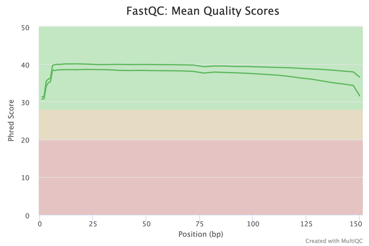
- How is the quality score over the reads? And the mean score?
- Is there any bias in base content?
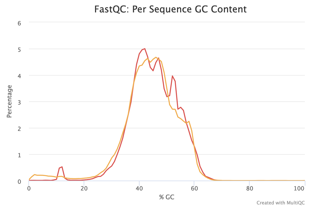
- How is the GC content?
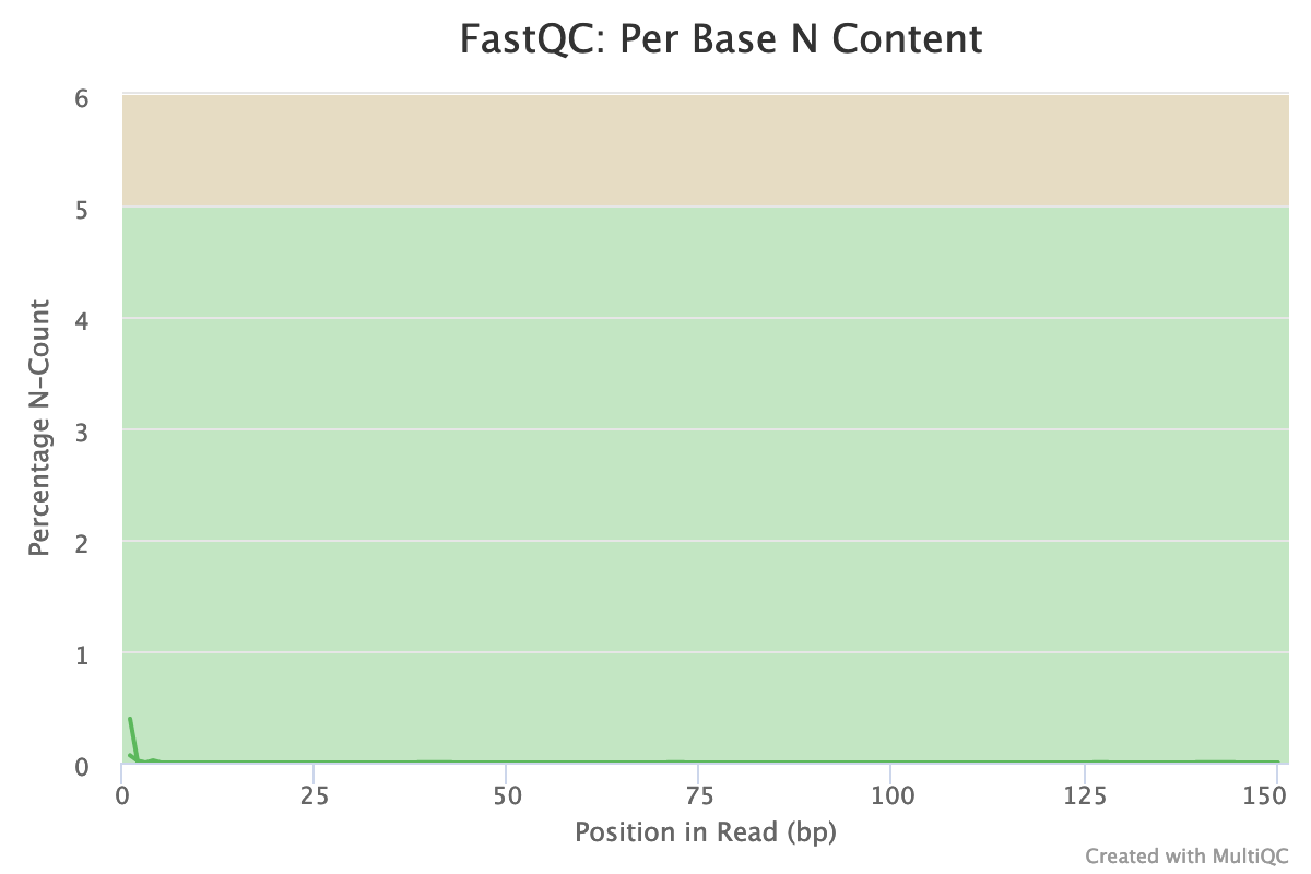
- Are there any unindentified bases?
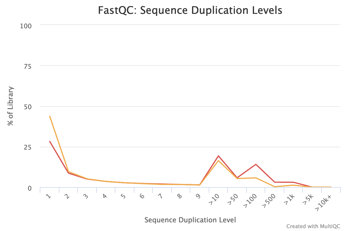
- Are there duplicated sequences?
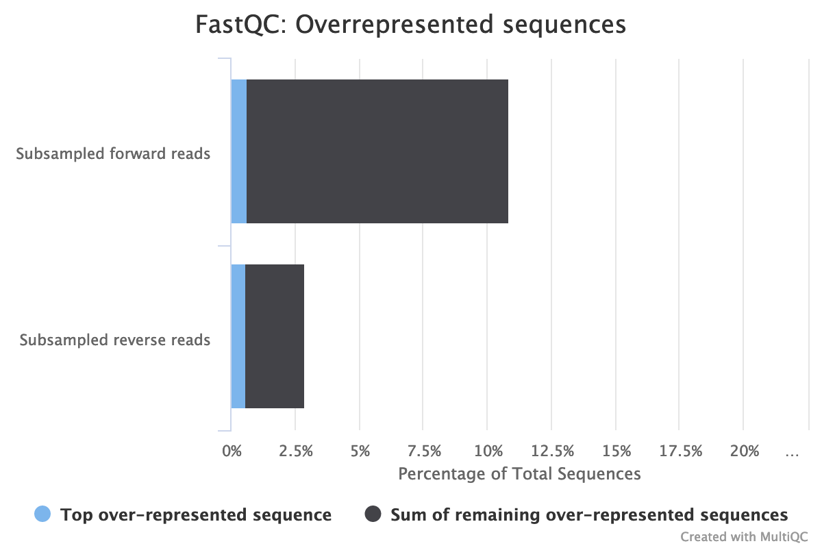
- Are there over-represented sequences?
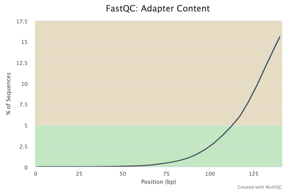
- Are there still some adapters left?
- What should we do next?
- Both files have 260,554 sequences
The “Per base sequence quality” is globally good: the quality stays around 40 over the reads, with just a slight decrease at the end (but still higher than 35)
The reverse reads have a slightly worse quality than the forward, a usual case in Illumina sequencing.
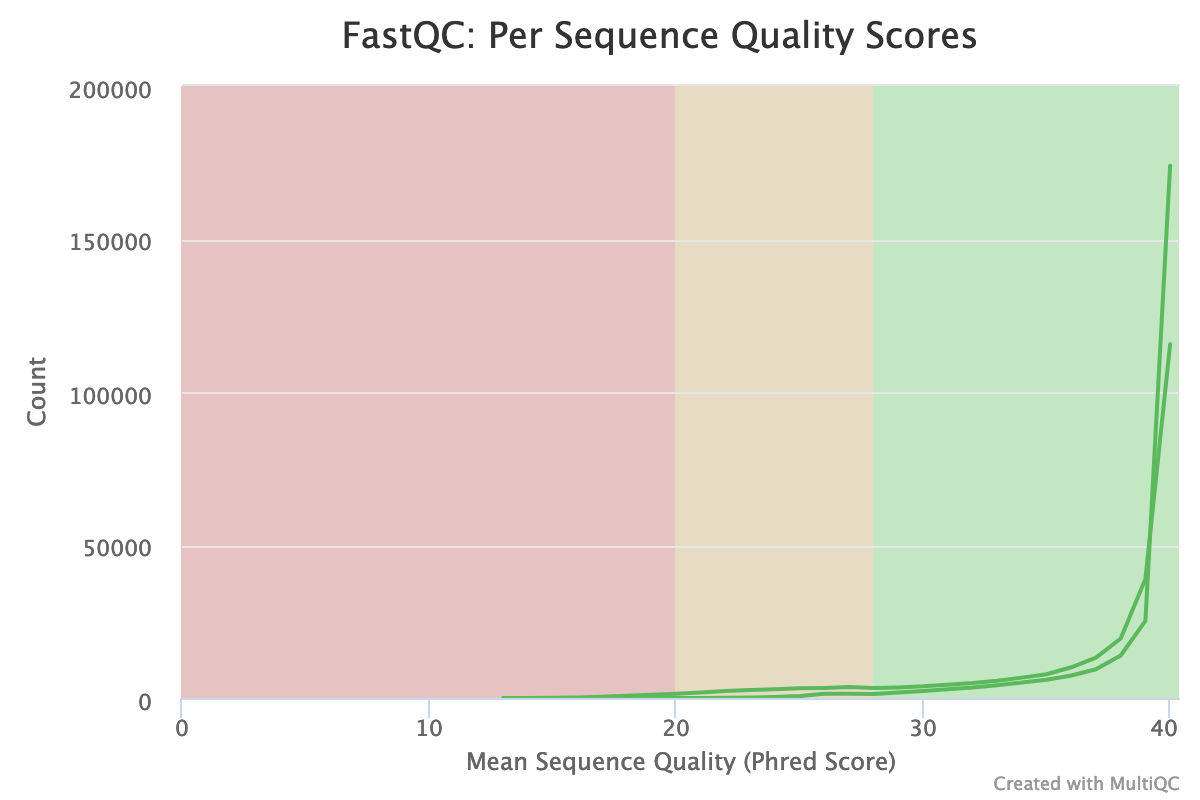
The distribution of the mean quality score is almost at the maximum for the forward and reverse reads:
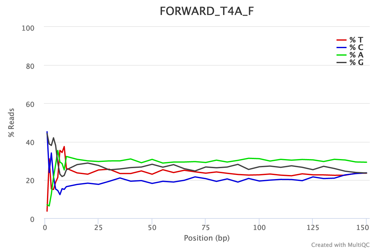
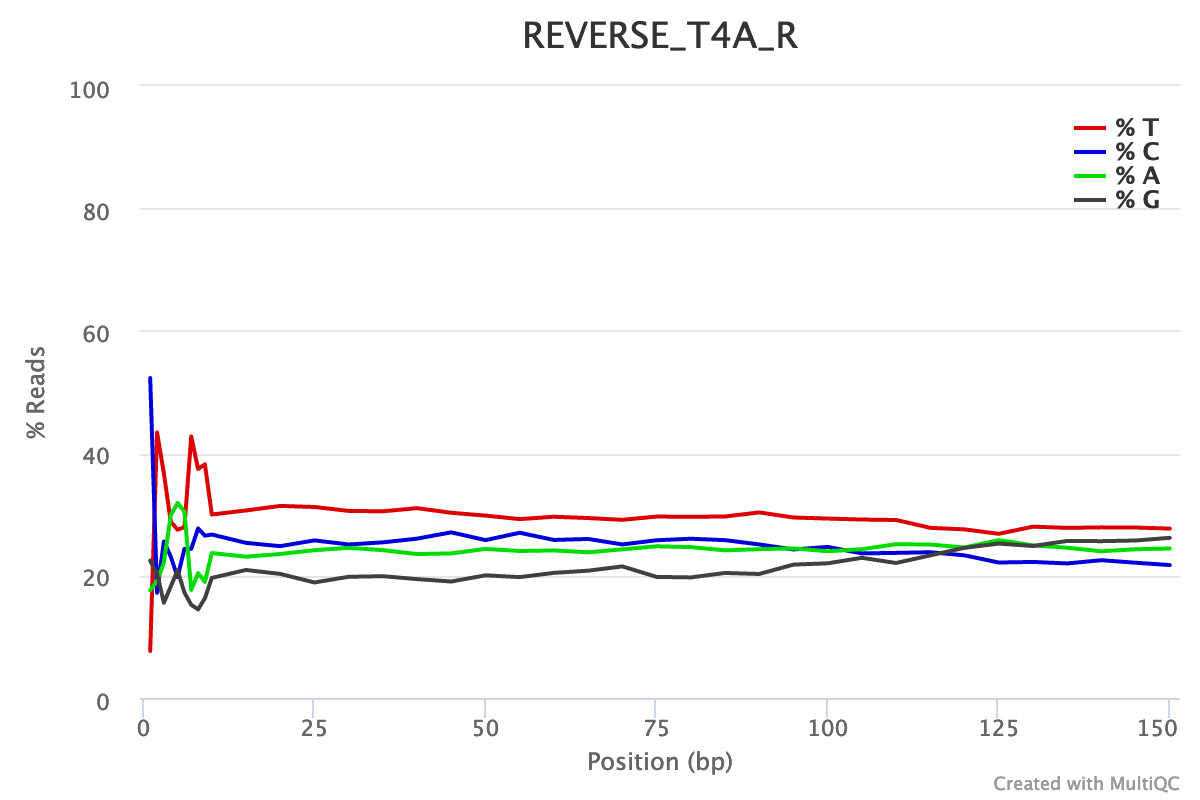
For both forward and reverse reads, the percentage of A, T, C, G over sequence length is biased. As for any RNA-seq data or more generally libraries produced by priming using random hexamers, the first 10-12 bases have an intrinsic bias.
We could also see that after these first bases the distinction between C-G and A-T groups is not clear as expected. It explains the error raised by FastQC.
With sequences from random position of a genome, we expect a normal distribution of the %GC of reads around the mean %GC of the genome. Here, we have RNA reads from various genomes. We do not expect a normal distribution of the %GC. Indeed, for the forward reads, the distribution shows with several peaks: maybe corresponding to mean %GC of different organisms.
Almost no N were found in the reads: so almost no unindentified bases
The forward reads seem to have more duplicated reads than the reverse reads with a rate of duplication up to 60% and some reads identified over 10 times.
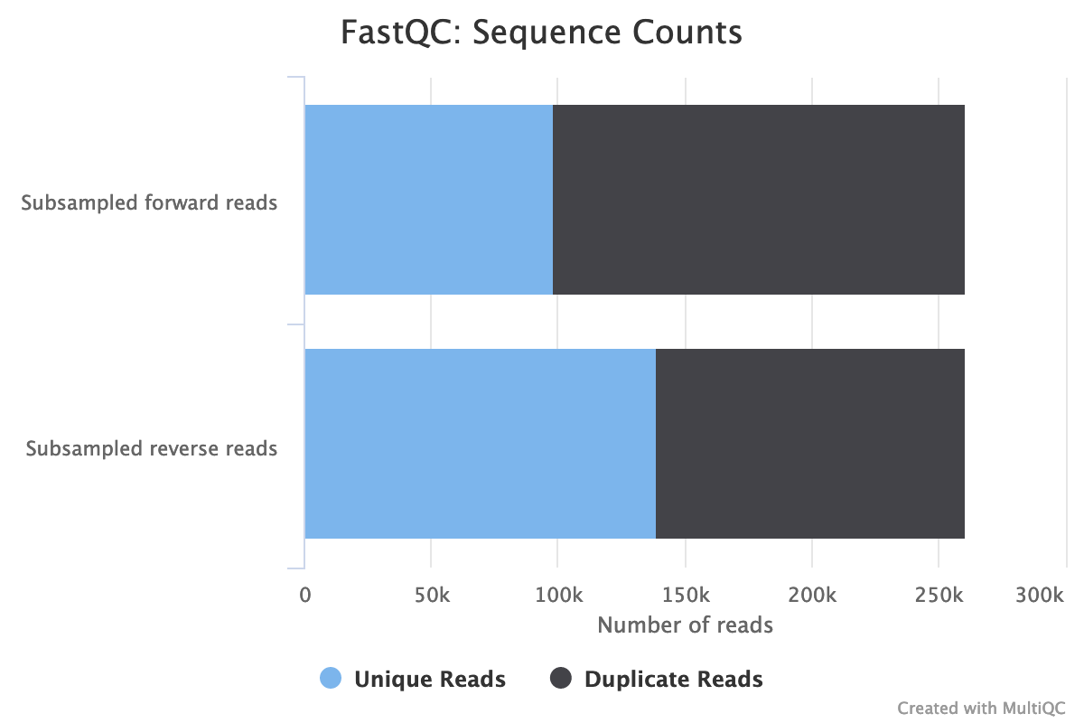
In data from RNA (metatranscriptomics data), duplicated reads are expected. The low rate of duplication in reverse reads could be due to bad quality: some nucleotides may have been wrongly identified, altering the reads and reducing the duplication.
The high rate of overrepresented sequences in the forward reads is linked to the high rate of duplication.
Illumina universal adapters are still present in the reads, especially at the 3’ end.
- After checking what is wrong, we should think about the errors reported by FastQC: they may come from the type of sequencing or what we sequenced (check the “Quality control” training: FastQC for more details): some like the duplication rate or the base content biases are due to the RNA sequencing. However, despite these challenges, we can still get slightly better sequences for the downstream analyses.
Even though our data is already of pretty high quality, we can improve it even more by:
- Trimming reads to remove sequencing adapters
- Trimming reads to remove bases that were sequenced with low certainty (= low-quality bases) at the ends of the reads
- Removing reads of overall bad quality
- Removing reads that are too short to be informative in downstream analysis
QuestionWhat are the possible tools to perform such functions?
There are many tools such as Cutadapt, Trimmomatic, Trim Galore, Clip, trim putative adapter sequences. etc. We choose here Cutadapt because it is error tolerant, it is fast and the version is pretty stable.
There are several tools out there that can perform these steps, but in this analysis we use Cutadapt (Martin 2011).
Cutadapt also helps find and remove adapter sequences, primers, poly-A tails and/or other unwanted sequences from the input FASTQ files. It trims the input reads by finding the adapter or primer sequences in an error-tolerant way. Additional features include modifying and filtering reads. We also add custom 3’ (end) adapter sequence cutting as suggested by Illumina.
Hands On: Read trimming and filtering
- Cutadapt ( Galaxy version 5.0+galaxy0) with the following parameters to trim low quality sequences:
- “Single-end or Paired-end reads?”:
Paired-end
- param-files “FASTQ/A file #1”:
T1A_forward- param-files “FASTQ/A file #2”:
T1A_reverseThe order is important here!
- In Read 1 Adapters
- 3’ (End) Adapters
- Click on param-repeat “3’ (End) Adapters”
- In 1: 3’ (End) Adapters
- Source:
Enter custom sequence- Custom 3’ adapter sequence:
AGATCGGAAGAGCACACGTCTGAACTCCAGTCA- In Read 2 Adapters
- 3’ (End) Adapters
- Click on param-repeat “3’ (End) Adapters”
- In 1: 3’ (End) Adapters
- Source:
Enter custom sequence- Custom 3’ adapter sequence:
AGATCGGAAGAGCGTCGTGTAGGGAAAGAGTGT- In “Other Read Trimming Options”
- “Quality cutoff(s) (R1)”:
20- In “Read Filtering Options”
- “Minimum length (R1)”:
150“Additional outputs to generate”:
ReportQuestionWhy do we run the trimming tool only once on a paired-end dataset and not twice, once for each dataset?
The tool can remove sequences if they become too short during the trimming process. For paired-end files it removes entire sequence pairs if one (or both) of the two reads became shorter than the set length cutoff. Reads of a read-pair that are longer than a given threshold but for which the partner read has become too short can optionally be written out to single-end files. This ensures that the information of a read pair is not lost entirely if only one read is of good quality.
- Rename galaxy-pencil
Read 1 outputtoQC controlled forward readsRead 2 outputtoQC controlled reverse reads
Cutadapt tool outputs a report file containing some information about the trimming and filtering it performed.
QuestionInspect the output report from Cutadapt tool.
- How many forward reads contained adapters? How many reverse reads?
- How many basepairs have been removed from the forward reads because of bad quality? And from the reverse reads?
- How many sequence pairs have been removed because at least one read was shorter than the length cutoff?
- How many sequence pairs written to files?
- 59,959 (23.0%) forward reads (read 1) with adapters, 57,069 (21.9%) reverse reads (read 2) with adapters
- 203,654 bp has been trimmed from the forward reads (read 1) and 569,653 bp from the reverse reads (read 2). It is not a surprise: we saw that at the end of the sequences the quality was dropping more for the reverse reads than for the forward reads.
- 84,276 (32.3%) reads were too short after trimming and then filtered.
- 176,278 sequence pairs
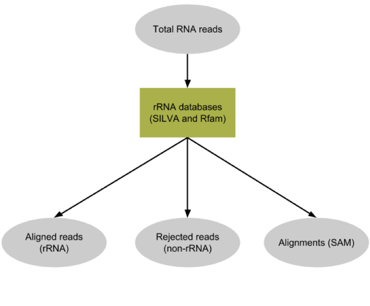
Ribosomal RNA fragments filtering
Metatranscriptomics sequencing targets any RNA in a pool of micro-organisms. In total RNA, the highest proportion of RNA sequences in any organism will be ribosomal RNAs (>90%). These rRNAs are useful for the taxonomic assignment (i.e. which organisms are found) but they do not provide any functional information, (i.e. which genes are expressed). Here, rRNA reads were depleted experimentally to enrich the sample in sequences from mRNA. Still, the depletion is not perfect and there are some rRNA left (which taxonomic profile may be different from the original pool). To make the downstream functional annotation faster, we will sort the rRNA sequences using SortMeRNA (Kopylova et al. 2012). It can handle large RNA databases and sort out all fragments matching to the database with high accuracy and specificity:
Hands On: Ribosomal RNA fragments filtering
- Filter with SortMeRNA ( Galaxy version 4.3.6+galaxy0) with the following parameters:
- “Sequencing type”:
Paired-end reads
- param-file “Forward reads”:
QC controlled forward reads(output of Cutadapt tool)- param-file “Reverse reads”:
QC controlled reverse reads(output of Cutadapt tool)- “If one of the paired-end reads aligns and the other one does not”:
Output both reads to rejected file (--paired_out)- “Databases to query”:
Public ribosomal databases
- “rRNA databases”: param-check Select all
- param-check
rfam-5s-database-id98- param-check
silva-arc-23s-id98- param-check
silva-euk-28s-id98- param-check
silva-bac-23s-id98- param-check
silva-euk-18s-id95- param-check
silva-bac-16s-id90- param-check
rfam-5.8s-database-id98- param-check
silva-arc-16s-id95- “Include aligned reads in FASTA/FASTQ format?”:
Yes (--fastx)
- “Include rejected reads file?”:
YesExpand the aligned and unaligned forward reads datasets in the history
QuestionHow many sequences have been identified as rRNA and non rRNA?
Answer normally from the log file … not available at the moment
SortMeRNA tool removes any reads identified as rRNA from our dataset, and output a log file (absent at the moment) with more information about this filtering. <!—
QuestionInspect the log output from SortMeRNA tool, and scroll down to the
Resultssection.
- How many reads have been processed?
- How many reads have been identified as rRNA given the log file?
352,556 reads are processed: 176,278 for forward and 176,278 for reverse (given the Cutadapt report)
Out of the 352,556 reads, xxx,xxx (x %) have passed the e-value threshold and are identified as rRNA.
Some of the aligned reads are forward (resp. reverse) reads but the corresponding reverse (resp. forward) reads are not aligned. As we choose “If one of the paired-end reads aligns and the other one does not”:
Output both reads to rejected file (--paired_out), if one read in a pair does not align, both go to unaligned.
–>
Interlace forward and reverse reads
The tool for functional annotations needs a single file as input, even with paired-end data.
We need to join the two separate files (forward and reverse) to create a single interleaced file, using FASTQ interlacer, in which the forward reads have /1 in their id and reverse reads /2. The join is performed using sequence identifiers (headers), allowing the two files to contain differing ordering. If a sequence identifier does not appear in both files, it is output in a separate file named singles.
We use FASTQ interlacer on the unaligned (non-rRNA) reads from SortMeRNA to prepare for the functional analysis.
Hands On: Interlace FastQ files
- FASTQ interlacer ( Galaxy version 1.2.0.1+galaxy0) with the following parameters:
- “Type of paired-end datasets”:
2 separate datasets
- param-file “Left-hand mates”:
Unaligned forward reads(output of SortMeRNA tool)- param-file “Right-hand mates”:
Unaligned reverse reads(output of SortMeRNA tool)- Rename galaxy-pencil the pair output to
Interlaced non rRNA reads
QuestionHow many pairs have been interlaced?
133,910 pairs of sequence have been written to file
Extraction of the community profile
exchange Switch to short tutorial
The first important information to get from microbiome data is the community structure: which organisms are present and in which abundance. This is called taxonomic profiling.
Different approaches can be used:
-
Identification and classification of Operational Taxonomic Units OTUs, as used in amplicon data
Such an approach first requires sequence sorting to extract only the 16S and 18S sequences (e.g. using aligned reads from SortMeRNA when rRNAs have not been depleted experimentally), then again using the same tools as for amplicon data (as explained in tutorials like 16S Microbial Analysis with mothur or 16S Microbial analysis with Nanopore data).
-
Assignment of taxonomy on the whole sequences using databases with marker genes
In this tutorial, we follow second approach using MetaPhlAn (Truong et al. 2015). This tool uses a database of ~1M unique clade-specific marker genes (not only the rRNA genes) identified from ~17,000 reference (bacterial, archeal, viral and eukaryotic) genomes.
Hands On: Extract the community structure
- MetaPhlAn ( Galaxy version 4.1.1+galaxy4) with the following parameters:
- In “Input(s)”
- “Input(s)”:
Fasta/FastQ file(s) with microbiota reads
- “Fasta/FastQ file(s) with microbiota reads”:
Paired-end files
- param-file “Forward paired-end Fasta/FastQ file with microbiota reads”:
Unaligned forward reads(output of SortMeRNA tool)- param-file “Reverse paired-end Fasta/FastQ file with microbiota reads”:
Unaligned reverse reads(output of SortMeRNA tool)- “Database with clade-specific marker genes”:
Locally cached
- “Cached database with clade-specific marker genes”:
MetaPhlAn clade-specific marker genes (mpa_vJune23_CHOCOPhlAn_202403)- In “Analysis”
- “Type of analysis to perform”:
rel_ab: Profiling a metagenomes in terms of relative abundances
- “Taxonomic level for the relative abundance output”:
All taxonomic levels- *“Generate a report for each taxonomic level?”:
Yes- “Quantile value for the robust average”:
0.1- “Organisms to profile”:
- param-check
Profile viral organisms (add_viruses)- In “Output”
- “Output for Krona”:
Yes
This step may take a couple of minutes as each sequence is compare to the full database with ~1 million reference sequences.
5 files and a collection are generated by MetaPhlAn tool:
-
The main output: A tabular file called
Predicted taxon relative abundanceswith the *community profile#mpa_vJun23_CHOCOPhlAnSGB_202403 # ... #465754 reads processed #SampleID Metaphlan_Analysis #clade_name NCBI_tax_id relative_abundance additional_species k__Bacteria 2 100.0 k__Bacteria|p__Firmicutes 2|1239 71.87781 k__Bacteria|p__Coprothermobacterota 2|2138240 28.12219 k__Bacteria|p__Firmicutes|c__Clostridia 2|1239|186801 71.87781 k__Bacteria|p__Coprothermobacterota|c__Coprothermobacteria 2|2138240|2138243 28.12219 k__Bacteria|p__Firmicutes|c__Clostridia|o__Eubacteriales 2|1239|186801|186802 71.87781 k__Bacteria|p__Coprothermobacterota|c__Coprothermobacteria|o__Coprothermobacterales 2|2138240|2138243|2138246 28.12219 k__Bacteria|p__Firmicutes|c__Clostridia|o__Eubacteriales|f__Oscillospiraceae 2|1239|186801|186802|216572 71.87781 k__Bacteria|p__Coprothermobacterota|c__Coprothermobacteria|o__Coprothermobacterales|f__Coprothermobacteraceae 2|2138240|2138243|2138246|2138247Each line contains 4 columns:
- the lineage with different taxonomic levels
- the previous lineage with NCBI taxon id
- the relative abundance found for our sample for the lineage
- any additional species
The file starts with high level taxa (kingdom:
k__) and go to more precise taxa.QuestionInspect the
Predicted taxon relative abundancesfile output by MetaPhlAn tool- How many taxons have been identified?
- What are the different taxonomic levels we have access to with MetaPhlAn?
- What genus and species are found in our sample?
- Has only bacteria been identified in our sample?
- The file has 15 lines. Therefore, 15 taxons of different levels have been identified
- We have access: kingdom (
k__), phylum (p__), class (c__), order (o__), family (f__), genus (g__), species (s__), strain (t__) - In our sample, we identified:
- 2 genera: Coprothermobacter, Acetivibrio
- 2 species: Coprothermobacter proteolyticus, Acetivibrio thermocellus
- The analysis shows indeed, that only bacteria can be found in our sample.
- A collection with the same information as in the tabular file but splitted into different files, one per taxonomic level
- A tabular file called
Predicted taxon relative abundances for Kronawith the same information as the previous file but formatted for visualization using Krona. We will use this file later -
A BIOM file with the same information as the previous file but in BIOM format
BIOM format is quite common in microbiomics. This is standard, for example, as the input for tools like mothur or QIIME.
- A SAM file with the results of the sequence mapping on the reference database.
- A tabular file called
Bowtie2 outputwith similar information as the one in the SAM file
Comment: Analyzing an isolated metatranscriptomeWe are analyzing our RNA reads as we would do for DNA reads. This approach has one main caveat. In MetaPhlAn, the species are quantified based on the recruitment of reads to species-specific marker genes. In metagenomic data, each genome copy is assumed to donate ~1 copy of each marker. But the same assumption cannot be made for RNA data: markers may be transcribed more or less within a given species in this sample compared to the average transcription rate. A species will still be detected in the metatranscriptomic data as long as a non-trivial fraction of the species’ markers is expressed.
We should then carefully interpret the species relative abundance. These values reflect species’ relative contributions to the pool of species-specific transcripts and not the overall transcript pool.
Some downstream tools need the MetaPhlAn table with predicted taxon abundance with only 2 columns: the lineage and the abundance.
Hands On: Format taxon relative abundances table
- Cut with the following parameters:
- “Cut columns”:
c1,c3- param-file “From”:
Predicted taxon relative abundances(output of MetaPhlAn)- Rename
Cut predicted taxon relative abundances table
Community structure visualization
Even if the output of MetaPhlAn can be easy to parse, we want to visualize and explore the community structure. 2 tools can be used there:
- Krona for an interactive HTML output
- Graphlan for a publication ready visualization
Hands On: Interactive community structure visualization with KRONA
- Krona pie chart ( Galaxy version 2.7.1+galaxy0) with
- “What is the type of your input data”:
Tabular
- param-file “Input file”:
Predicted taxon relative abundances for Krona(output of MetaPhlAn)
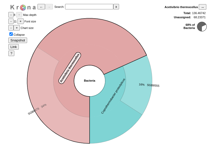
Krona Ondov et al. 2011 renders results of a metagenomic profiling as a zoomable pie chart. It allows hierarchical data, here taxonomic levels, to be explored with zooming, multi-layered pie charts
QuestionInspect the output from Krona tool. (The interactive plot is also shown below)
- What are the abundances of the 2 bacterial subclasses identified here?
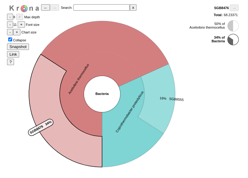
- When zooming on Acetivibrio thermocellus, what are the abundances of the specific strain ?
Acetivibrio thermocellus represents 72% and Coprothermobacter proteolyticus 28% of the bacteria identified in our sample
50% of bacteria are from the strain SGB8476.
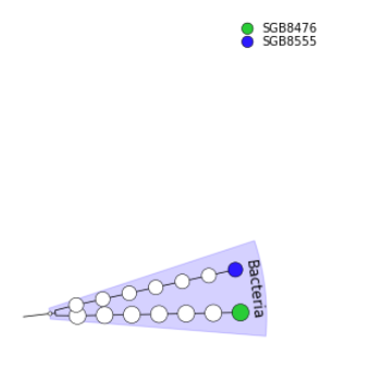
GraPhlAn is another software tool for producing high-quality circular representations of taxonomic and phylogenetic trees.
It takes a taxonomic tree file as the input. We first need to convert the MetaPhlAn output using Export to GraPhlAn. This conversion software tool produces both annotation and tree file for GraPhlAn.
Hands On: Publication-ready community structure visualization with GraPhlAn
- Export to GraPhlAn ( Galaxy version 0.20+galaxy0) with the following parameters:
- param-file “Input file”:
Cut predicted taxon relative abundances table- “List which levels should be annotated in the tree”:
1,2- “List which levels should use the external legend for the annotation”:
3,4,5- “List which levels should be highlight with a shaded background”:
1- Generation, personalization and annotation of tree ( Galaxy version 1.1.3) with the following parameters:
- param-file “Input tree”:
Tree(output of Export to GraPhlAn)- param-file “Annotation file”:
Annotation(output of Export to GraPhlAn)- GraPhlAn ( Galaxy version 1.1.3) with the following parameters:
- param-file “Input tree”:
Tree in PhyloXML- “Output format”:
PNG- Inspect GraPhlAn output
Extract the functional information
exchange Switch to short tutorial
We would now like to answer the question “What are the micro-organisms doing?” or “Which functions are performed by the micro-organisms in the environment?”.
In the metatranscriptomics data, we have access to the genes that are expressed by the community. We can use that to identify genes, assing their functions, and build pathways, etc., to investigate their contribution to the community using HUMAnN (Franzosa et al. 2018). HUMAnN is a pipeline developed for efficiently and accurately profiling the presence/absence and abundance of microbial pathways in a community from metagenomic or metatranscriptomic sequencing data.
To identify the functions made by the community, we do not need the rRNA sequences, since they do not contain gene coding regions and will slow the run. We will use the output of SortMeRNA, but also the identified community profile from MetaPhlAn. This will help HUMAnN to focus on the known sequences for the identified organisms.
Hands On: Extract the functional information
- HUMAnN ( Galaxy version 3.9+galaxy0) with the following parameters:
- “Input(s)”:
Quality-controlled shotgun sequencing reads (metagenome (DNA reads) or metatranscriptome (RNA reads))
- param-file “Quality-controlled shotgun sequencing reads (metagenome (DNA reads) or metatranscriptome (RNA reads))”:
Interlaced non rRNA reads- “Steps”:
Bypass the taxonomic profiling step and creates a custom ChocoPhlAn database of the species provided afterwards
- param-file“Taxonomic profile file”:
Predicted taxon relative abundances(output of MetaPhlAn tool)- In “Nucleotide search / Mapping reads to community pangenomes”
- “Nucleotide database”:
Locally cached
- “Nucleotide database”:
Full ChocoPhlAn for HUMAnN- In “Translated search / Aligning unmapped reads to a protein database”
- “Protein database”:
Locally cached
- “Protein database”:
Full UniRef90 for HUMAnN
Import the 2 files:
https://zenodo.org/record/4776250/files/T1A_HUMAnN_Gene_families_and_their_abundance.tabular
https://zenodo.org/record/4776250/files/T1A_HUMAnN_Pathways_and_their_abundance.tabular
HUMAnN tool generates 4 files:
-
A tabular file with the gene families and their abundance:
 # Gene Family 	humann_Abundance-RPKs
 UNMAPPED 	93840.0000000000
 UniRef90_A3DCI4 	42213.2661898446
 UniRef90_A3DCI4|g__Hungateiclostridium.s__Hungateiclostridium_thermocellum 	42205.5707425926
 UniRef90_A3DCI4|unclassified 	7.6954472520
 UniRef90_A3DCB9 	39287.6314397701
 UniRef90_A3DCB9|g__Hungateiclostridium.s__Hungateiclostridium_thermocellum 	39273.2031556915
 UniRef90_A3DCB9|unclassified 	14.4282840786
 UniRef90_A3DC67 	33183.8388613174
This file details the abundance of each gene family in the community. Gene families are groups of evolutionarily-related protein-coding sequences that often perform similar functions. Here we used UniRef90 gene families: sequences in a gene family have at least 90% sequence identity.
Gene family abundance at the community level is stratified to show the contributions from known and unknown species. Individual species’ abundance contributions sum to the community total abundance.
Gene family abundance is reported in RPK (reads per kilobase) units to normalize for gene length. It reflects the relative gene (or transcript) copy number in the community.
The “UNMAPPED” value is the total number of reads which remain unmapped after both alignment steps (nucleotide and translated search). Since other gene features in the table are quantified in RPK units, “UNMAPPED” can be interpreted as a single unknown gene of length 1 kilobase recruiting all reads that failed to map to known sequences.
QuestionInspect the
Gene families and their abundancesfile from HUMAnN tool- What is the most abundant family?
- Which species is involved in production of this family?
- How many gene families have been identified?
- The most abundant family is the first one in the family: UniRef90_A3DCI4. We can use the tool Rename features of a HUMAnN generated table ( Galaxy version 3.9+galaxy0) to add extra information about the gene family.
- “Type of feature renaming”:
Advanced feature renaming - “Features to be renamed”:
Mapping (full) between UniRef90 ids and names
- “Type of feature renaming”:
- This family is mapped to Hungateiclostridium thermocellum, which is consistent with information from UniRef90 gene families: the (2Fe-2S) ferredoxin domain-containing protein seems to be produced mostly by Hungateiclostridium thermocellum.
-
There is 6,401 lines in gene family file. But some of the gene families have multiple lines when the involved species are known.
To know the number of gene families, we need to remove all lines with the species information, i.e. lines with
|in them using the tool Split a HUMAnN table ( Galaxy version 3.9+galaxy0)The tool generates 2 output file:
- a stratified table with all lines with
|in them - a unstratied table with all lines without
|in them
In the unstratified table, there are 3,189 lines, so 3,188 gene families.
- a stratified table with all lines with
-
A tabular file with the pathways and their abundance:
 # Pathway 	humann_Abundance
 UNMAPPED 	8327.1254237651
 UNINTEGRATED 	48674.2486093581
 UNINTEGRATED|g__Hungateiclostridium.s__Hungateiclostridium_thermocellum 	29349.2544670158
 UNINTEGRATED|unclassified 	3154.6737904970
 PWY-6609: adenine and adenosine salvage III 	274.2550568127
 PWY-6609: adenine and adenosine salvage III|g__Hungateiclostridium.s__Hungateiclostridium_thermocellum 	66.3688569288
 PWY-6609: adenine and adenosine salvage III|unclassified 	8.0057395198
 PWY-1042: glycolysis IV 	194.2215953218
This file shows each pathway and their abundance. Here, we used the MetaCyc Metabolic Pathway Database, a curated database of experimentally elucidated metabolic pathways from all domains of life.
The abundance of a pathway in the sample is computed as a function of the abundances of the pathway’s component reactions, with each reaction’s abundance computed as the sum over abundances of genes catalyzing the reaction. The abundance is proportional to the number of complete “copies” of the pathway in the community. Indeed, for a simple linear pathway
RXN1 --> RXN2 --> RXN3 --> RXN4, if RXN1 is 10 times as abundant as RXNs 2-4, the pathway abundance will be driven by the abundances of RXNs 2-4.The pathway abundance is computed once for all species (community level) and again for each species using species gene abundances along the components of the pathway. Unlike gene abundance, a pathway’s abundance at community-level is not necessarily the sum of the abundance values of each species. For example, for the same pathway example as above, if the abundances of RXNs 1-4 are [5, 5, 10, 10] in Species A and [10, 10, 5, 5] in Species B, the pathway abundance would be 5 for Species A and Species B, but 15 at the community level as the reaction totals are [15, 15, 15, 15].
QuestionView the
Pathways and their abundanceoutput from HUMAnN tool- What is the most abundant pathway?
- Which species is involved in production of this pathway?
- How many pathways have been identified?
- What is the “UNINTEGRATED” abundance?
- The most abundant pathway is PWY-6609. It produces the adenine and adenosine salvage III.
- Like the gene family, this pathway is mostly achieved by Hungateiclostridium thermocellum.
-
There are 117 lines in the pathway file, including the lines with species information. To compute the number of pathways, we need to apply a similar approach as for the gene families by removing the lines with
|in them using the tool Split a HUMAnN table ( Galaxy version 3.9+galaxy0). The unstratified output file has 63 lines, including the header, UNMAPPED and UNINTEGRATED. Therefore, 60 MetaCyc pathways have been identified for our sample. - The “UNINTEGRATED” abundance corresponds to the total abundance of genes in the different levels that do not contribute to any pathways.
-
A file with the pathways and their coverage:
Pathway coverage provides an alternative description of the presence (1) and absence (0) of pathways in a community, independent of their quantitative abundance.
-
A log file
Comment: Analyzing an isolated metatranscriptomeAs we already mentioned above, we are analyzing our RNA reads as we would do for DNA reads and therefore we should be careful when interpreting the results. We already mentioned the analysis of the species’ relative abundance from MetaPhlAn, but there is another aspect we should be careful about.
From a lone metatranscriptomic dataset, the transcript abundance can be confounded with the underlying gene copy number. For example, transcript X may be more abundant in sample A relative to sample B because the underlying X gene (same number in both samples) is more highly expressed in sample A relative to sample B; or there are more copies of gene X in sample A relative to sample B (all of which are equally expressed). This is a general challenge in analyzing isolated metatranscriptomes.
The best approach would be to combine the metatranscriptomic analysis with a metagenomic analysis. In this case, rather than running MetaPhlAn on the metatranscriptomic data, we run it on the metagenomic data and use the taxonomic profile as input to HUMAnN. RNA reads are then mapped to any species’ pangenomes detected in the metagenome. Then we run HUMAnN on both metagenomics and metatranscriptomic data. We can use both outputs to normalize the RNA-level outputs (e.g. transcript family abundance) by corresponding DNA-level outputs to the quantification of microbial expression independent of gene copy number.
Here we do not have a metagenomic dataset to combine with and need to be careful in our interpretation.
Normalize the abundances
Gene family and pathway abundances are in RPKs (reads per kilobase), accounting for gene length but not sample sequencing depth. While there are some applications, e.g. strain profiling, where RPK units are superior to depth-normalized units, most of the time we need to renormalize our samples prior to downstream analysis.
Hands On: Normalize the gene family abundances
- Renormalize a HUMAnN generated table ( Galaxy version 3.9+galaxy0) with
- “Gene/pathway table”:
Gene families and their abundance(output of HUMAnN)- “Normalization scheme”:
Relative abundance- “Normalization level”:
Normalization of all levels by community total- Rename galaxy-pencil the generated file
Normalized gene families
QuestionInspect galaxy-eye the
Normalized gene familiesfile
- What percentage of sequences has not been assigned to a gene family?
- What is the relative abundance of the most abundant gene family?
- 13.9% (\(0.138318 x 100\)) of the sequences have not be assigned to a gene family.
- The UniRef90_A3DCI4 family represents 6.22% of the reads.
Let’s do the same for the pathway abundances.
Hands On: Normalize the pathway abundances
- Renormalize a HUMAnN generated table ( Galaxy version 3.9+galaxy0) with
- “Gene/pathway table”:
Pathways and their abundance(output of HUMAnN)- “Normalization scheme”:
Relative abundance- “Normalization level”:
Normalization of all levels by community total- Rename galaxy-pencil the generated file
Normalized pathways
QuestionInspect galaxy-eye the
Normalized pathwaysfile.
- What is the UNMAPPED percentage?
- What percentage of reads assigned to a gene family has not be assigned to a pathway?
- What is the relative abundance of the most abundant gene family?
- UNMAPPED, here 13.9% of the reads, corresponds to the percentage of reads not assigned to gene families. It is the same value as in the normalized gene family file.
- 81% (UNINTEGRATED) of reads assigned to a gene family have not be assigned to a pathway
- The PWY-6609 pathway represents 0.46% of the reads.
Identify the gene families involved in the pathways
We would like to know which gene families are involved in our most abundant pathways and which species. For this, we use the tool Unpack pathway abundances to show genes included tool from HUMAnN tool suites.
Hands On: Normalize the gene family abundances
- Unpack pathway abundances to show genes included ( Galaxy version 3.9+galaxy0) with
- “Gene family or EC abundance file”:
Normalized gene families- “Pathway abundance file”:
Normalized pathways
This tool unpacks the pathways to show the genes for each. It adds another level of stratification to the pathway abundance table by including the gene family abundances:
# Pathway 	humann_Abundance-RELAB
ANAGLYCOLYSIS-PWY: glycolysis III (from glucose) 	0.000887968
ARO-PWY: chorismate biosynthesis I 	0.000703087
ARO-PWY|g__Hungateiclostridium.s__Hungateiclostridium_thermocellum 	0.000703087
ARO-PWY|g__Hungateiclostridium.s__Hungateiclostridium_thermocellum|UniRef90_A3DDJ2 	4.73896e-05
ARO-PWY|g__Hungateiclostridium.s__Hungateiclostridium_thermocellum|UniRef90_A0A1E3C026 	8.27656e-05
ARO-PWY|g__Hungateiclostridium.s__Hungateiclostridium_thermocellum|UniRef90_A3DDD8
QuestionInspect galaxy-eye the output from Unpack pathway abundances to show genes included tool
Which gene families are involved in the PWY-6609 pathway (the most abundant one)? And which species?
If we search the generated file for (using CTRF or CMDF):
PWY-6609: adenine and adenosine salvage III 	0.00455552
PWY-6609|g__Hungateiclostridium.s__Hungateiclostridium_thermocellum 	0.00110242
PWY-6609|g__Hungateiclostridium.s__Hungateiclostridium_thermocellum|UniRef90_A3DHM7 	0.00023651
PWY-6609|g__Hungateiclostridium.s__Hungateiclostridium_thermocellum|UniRef90_A3DD28 	4.48733e-05
PWY-6609|g__Hungateiclostridium.s__Hungateiclostridium_thermocellum|UniRef90_A3DEQ4 	3.69581e-05
PWY-6609|unclassified 	0.000132979
PWY-6609|unclassified|UniRef90_A0A140L1V2 	5.93149e-06
PWY-6609|unclassified|UniRef90_B5Y8G4 	0.001116
The gene families UniRef90_A3DD28, UniRef90_A3DHM7 and UniRef90_A3DEQ4 are identified, for Hungateiclostridium thermocellum, and UniRef90_A0A140L1V2 and UniRef90_B5Y8G4 for no species.
Group gene families into GO terms
The gene families can be a long list of ids and going through the gene families one by one to identify the interesting ones can be cumbersome. To help construct a big picture, we could identify and use categories of genes using the gene families.
Gene Ontology (GO) analysis is widely used to reduce complexity and highlight biological processes in genome-wide expression studies. There is a dedicated tool which groups and converts UniRef50 gene family abundances generated with HUMAnN into GO terms.
Hands On: Group abundances into GO terms
- Regroup HUMAnN table features ( Galaxy version 3.9+galaxy0) with the following parameters:
- param-file “Gene families table”:
Gene families and their abundance(output of HUMAnN)- “How to combine grouped features?”:
Sum- “Grouping”:
Grouping with larger mapping
- “Mapping to use for the grouping”:
Mapping (full) for Gene Ontology (GO) from UniRef90
The output is a table with the GO terms, their abundance and the involved species:
# Gene Family 	humann_Abundance-RPKs
UNMAPPED 	93840.0
UNGROUPED 	176772.794
UNGROUPED|g__Coprothermobacter.s__Coprothermobacter_proteolyticus 	4855.381
UNGROUPED|g__Hungateiclostridium.s__Hungateiclostridium_thermocellum 	152085.853
UNGROUPED|unclassified 	19831.56
GO:0000015 	250.882
GO:0000015|g__Coprothermobacter.s__Coprothermobacter_proteolyticus 	11.313
GO:0000015|g__Hungateiclostridium.s__Hungateiclostridium_thermocellum 	239.568
GO:0000027 	228.928
QuestionHow many GO term have been identified?
Using the tool Split a HUMAnN table ( Galaxy version 3.9+galaxy0), we see that the unstratified table has 1,175 lines (including the UNMAPPED, UNGROUPED and the header). So 1,172 GO terms have been identified.
The GO terms with their id are quite cryptic. We can rename them and then split them in 3 groups (molecular functions [MF], biological processes [BP] and cellular components [CC])
Hands On: Rename GO terms
- Rename features of a HUMAnN generated table ( Galaxy version 3.9+galaxy0) with the following parameters:
- param-file “Gene families table”: output of Regroup HUMAnN table features
- “Type of feature renaming”:
Advanced feature renaming
- “Features to be renamed”:
Mapping (full) between Gene Ontology (GO) ids and names- Select lines that match an expression with the following parameters:
- param-file “Select lines from”: output of last Rename features of a HUMAnN generated table
- “that”:
Matching- “the pattern”:
\[CC\]Rename galaxy-pencil the generated file
[CC] GO terms and their abundance- Select lines that match an expression with the following parameters:
- param-file “Select lines from”: output of last Rename features of a HUMAnN generated table
- “that”:
Matching- “the pattern”:
\[MF\]Rename galaxy-pencil the generated file
[MF] GO terms and their abundance- Select lines that match an expression with the following parameters:
- param-file “Select lines from”: output of last Rename features of a HUMAnN generated table
- “that”:
Matching- “the pattern”:
\[BP\]- Rename galaxy-pencil the generated file
[BP] GO terms and their abundance
QuestionInspect galaxy-eye the 3 outputs of these steps
- How many GO terms have been identified?
- Which of the GO terms related to molecular functions is the most abundant?
- After running Split a HUMAnN table ( Galaxy version 3.9+galaxy0) on the 3 outputs, we found:
- 412 BP GO terms
- 696 MF GO terms
- 58 CC GO terms
The GO terms in the
[MF] GO terms and their abundancefile are not sorted by abundance:GO:0000030: [MF] mannosyltransferase activity 16.321 GO:0000030: [MF] mannosyltransferase activity|g__Hungateiclostridium.s__Hungateiclostridium_thermocellum 16.321 GO:0000036: [MF] acyl carrier activity 726.24 GO:0000036: [MF] acyl carrier activity|g__Coprothermobacter.s__Coprothermobacter_proteolyticus 10.101 GO:0000036: [MF] acyl carrier activity|g__Hungateiclostridium.s__Hungateiclostridium_thermocellum 572.281So to identify the most abundant GO terms, we first need to sort the file using the Sort data in ascending or descending order ( Galaxy version 9.5+galaxy2) tool (on column 2, in descending order):
GO:0015035: [MF] protein disulfide oxidoreductase activity 	42923.275
GO:0015035: [MF] protein disulfide oxidoreductase activity|g__Hungateiclostridium.s__Hungateiclostridium_thermocellum 	40534.721
GO:0005524: [MF] ATP binding 	36370.768
GO:0003735: [MF] structural constituent of ribosome 	34810.272
GO:0046872: [MF] metal ion binding 	31185.883
GO:0005524: [MF] ATP binding|g__Hungateiclostridium.s__Hungateiclostridium_thermocellum 	30477.686
The most abundant GO terms related to molecular functions seem to be linked to protein disulfide oxidoreductase activity, but also to structural constituent of ribosome and ATP and metal ion binding.
Combine taxonomic and functional information
With MetaPhlAn and HUMAnN, we investigated “Which micro-organims are present in my sample?” and “What functions are performed by the micro-organisms in my sample?”. We can go further in these analyses, for example using a combination of functional and taxonomic results. Although we did not detail that in this tutorial you can find more methods of analysis in our tutorials on shotgun metagenomic data analysis.
Although gene families and pathways, and their abundance may be related to a species, in the HUMAnN output, relative abundance of the species is not indicated. Therefore, for each gene family/pathway and the corresponding taxonomic stratification, we will now extract the relative abundance of this gene family/pathway and the relative abundance of the corresponding species and genus.
Comment: Disagreement between MetaPhlAn and HUMAnN databaseWhen updating this tutorial we found, that in the combined table we can only find the species
Coprothermobacter_proteolyticus, although we know from the HUMAnN output that most gene families are associated to the species ofHungateiclostridium_thermocellum. An inspection of the uniprot entry showed, that the scientific name of Hungateiclostridium thermocellum is Acetivibrio thermocellus, which is the most abundant species found by MetaPhlAn. It can therefore be assumed, that the databases for HUMAnN and MetaPhlAn are not yet synchronized for all updates of taxonomic names. Hence, the gene family abundancy of the speciesHungateiclostridium_thermocellumfrom the HUMAnN output cannot be combined with the species abundancy of the MetaPhlAn output due to different naming conventions. To overcome this discrepancy, the naming ofHungateiclostridium_thermocellummust be changed in the HUMAnN output, this can be done with:
- Replace parts of text ( Galaxy version 1.1.4) with the following parameters:
- param-file “File to process”:
Normalized gene families- “Find and Replace”:
- “Find pattern”:
g__Hungateiclostridium.s__Hungateiclostridium_thermocellum- “Replace with”:
g__Acetivibrio.s__Acetivibrio_thermocellus- Rename galaxy-pencil the generated file
Normalized gene families adapted taxon
Hands On: Combine taxonomic and functional information
- Combine MetaPhlAn2 and HUMAnN2 outputs ( Galaxy version 0.3.0) with the following parameters:
- param-file “Input file corresponding to MetaPhlAN output”:
Predicted taxon relative abundances(output of MetaPhlAn tool)- param-file “Input file corresponding HUMAnN output”:
Normalized gene families adapted taxon- “Type of characteristics in HUMAnN file”:
Gene families- Inspect the generated file
The generated file is a table with 7 columns:
- genus
- abundance of the genus (percentage)
- species
- abundance of the species (percentage)
- gene family id
- gene family name
- gene family abundance (percentage)
genus 	genus_abundance 	species 	species_abundance 		gene_families_id 	gene_families_name 	gene_families_abundance
Acetivibrio 	71.87781 	Acetivibrio_thermocellus 	71.87781 	UniRef90_A3DCI4 		6.220988184186852
Acetivibrio 	71.87781 	Acetivibrio_thermocellus 	71.87781 	UniRef90_A3DCB9 		5.78876831034535
Acetivibrio 	71.87781 	Acetivibrio_thermocellus 	71.87781 	UniRef90_A3DC67 		4.889688572773241
Acetivibrio 	71.87781 	Acetivibrio_thermocellus 	71.87781 	UniRef90_A3DBR3 		3.4048190061843977
Acetivibrio 	71.87781 	Acetivibrio_thermocellus 	71.87781 	UniRef90_A3DI60 		2.9344691434724686
Acetivibrio 	71.87781 	Acetivibrio_thermocellus 	71.87781 	UniRef90_G2JC59 		2.6483592269836618
Acetivibrio 	71.87781 	Acetivibrio_thermocellus 	71.87781 	UniRef90_A3DEF8 		1.2948396220557343
Coprothermobacter 	28.12219 	Coprothermobacter_proteolyticus 	28.12219 	UniRef90_B5Y8J9 		0.949851722752528
Question
- Are there gene families associated with each genus identified with MetaPhlAn?
- How many gene families are associated to each genus?
- Are there gene families associated to each species identified with MetaPhlAn?
- How many gene families are associated to each species?
To answer the questions, we need to group the contents of the output of Combine MetaPhlAn and HUMAnN2 output by 1st column and count the number of occurrences of gene families. We do that using Group data by a column tool:
Hands On: Group by genus and count gene families
- Group data by a column
- “Select data”: output of Combine MetaPhlAn and HUMAnN outputs
- “Group by column”:
Column:1- “Operation”:
- Click on param-repeat “Insert Operation”
- “Type”:
Count- “On column”:
Column:5With MetaPhlAn, we identified 2 genus (Coprothermobacter and Acetivibrio). Both can be found in the combined output.
1,890 gene families are associated to Hungateiclostridium and 351 to Coprothermobacter.
For this question, we should group on the 3rd column:
Hands On: Group by species and count gene families
- Group data by a column
- “Select data”: output of Combine MetaPhlAn2 and HUMAnN2 outputs
- “Group by column”:
Column:3- “Operation”:
- Click on param-repeat “Insert Operation”
- “Type”:
Count- “On column”:
Column:5Similarely to the genus, 2 species (Coprothermobacter proteolyticus and Hungateiclostridium thermocellum) identified by MetaPhlAn are associated to gene families.
As the species found derived directly from the genus (not 2 species for the same genus here), the number of gene families identified are the sames: 351 for Coprothermobacter proteolyticus and 1,890 for Hungateiclostridium thermocellum.
We could now apply the same tool to the pathways and run similar analysis.
Conclusion
In this tutorial, we analyzed one metatranscriptomics sample from raw sequences to community structure, functional profiling. To do that, we:
- preprocessed the raw data: quality control, trimming and filtering, sequence sorting and formatting
-
extracted and analyzed the community structure (taxonomic information)
We identified bacteria to the level of strains, but also some archaea.
-
extracted and analyzed the community functions (functional information)
We extracted gene families, pathways, but also the gene families involved in pathways and aggregated the gene families into GO terms
- combined taxonomic and functional information to offer insights into taxonomic contribution to a function or functions expressed by a particular taxonomy
The workflow can be represented this way:
The dataset used here was extracted from a time-series analysis of a microbial community inside a bioreactor (Kunath et al. 2018) in which there are 3 replicates over 7 time points. We analyzed here only one single time point for one replicate.
You've Finished the Tutorial
Key points
Metatranscriptomics data have the same QC profile that RNA-seq data
A lot of metatranscriptomics sequences are identified as rRNA sequences
With shotgun data, we can extract information about the studied community structure and also the functions realised by the community
Metatranscriptomics data analyses are complex and must be careful done, specially when they are done without combination to metagenomics data analyses
Frequently Asked Questions
Have questions about this tutorial? Have a look at the available FAQ pages and support channelsUseful literature
Further information, including links to documentation and original publications, regarding the tools, analysis techniques and the interpretation of results described in this tutorial can be found here.
References
- Martin, M., 2011 Cutadapt removes adapter sequences from high-throughput sequencing reads. EMBnet. journal 17: 10–12. 10.14806/ej.17.1.200
- Ondov, B. D., N. H. Bergman, and A. M. Phillippy, 2011 Interactive metagenomic visualization in a Web browser. BMC bioinformatics 12: 385. 10.1186/1471-2105-12-385
- Kopylova, E., L. Noé, and H. Touzet, 2012 SortMeRNA: fast and accurate filtering of ribosomal RNAs in metatranscriptomic data. Bioinformatics 28: 3211–3217. 10.1093/bioinformatics/bts611
- Truong, D. T., E. A. Franzosa, T. L. Tickle, M. Scholz, G. Weingart et al., 2015 MetaPhlAn2 for enhanced metagenomic taxonomic profiling. Nature methods 12: 902. 10.1038/nmeth.3589
- Batut, B., K. Gravouil, C. Defois, S. Hiltemann, J.-F. Brugère et al., 2018 ASaiM: a Galaxy-based framework to analyze microbiota data. GigaScience 7: giy057. 10.1093/gigascience/giy057
- Franzosa, E. A., L. J. McIver, G. Rahnavard, L. R. Thompson, M. Schirmer et al., 2018 Species-level functional profiling of metagenomes and metatranscriptomes. Nature methods 15: 962. 10.1038/s41592-018-0176-y
- Kunath, B. J., F. Delogu, A. E. Naas, M. Ø. Arntzen, V. G. H. Eijsink et al., 2018 From proteins to polysaccharides: lifestyle and genetic evolution of Coprothermobacter proteolyticus. The ISME journal 1. 10.1038/s41396-018-0290-y
- Mehta, S., M. Crane, E. Leith, B. Batut, S. Hiltemann et al., 2021 ASaiM-MT: a validated and optimized ASaiM workflow for metatranscriptomics analysis within Galaxy framework: F1000Research 10:103. Type: article. 10.12688/f1000research.28608.2 https://f1000research.com/articles/10-103
Feedback
Did you use this material as an instructor? Feel free to give us feedback on how it went.
Did you use this material as a learner or student? Click the form below to leave feedback.

Citing this Tutorial
- Pratik Jagtap, Subina Mehta, Ray Sajulga, Bérénice Batut, Emma Leith, Praveen Kumar, Saskia Hiltemann, Metatranscriptomics analysis using microbiome RNA-seq data (Galaxy Training Materials). https://training.galaxyproject.org/training-material/topics/microbiome/tutorials/metatranscriptomics/tutorial.html Online; accessed TODAY
- Hiltemann, Saskia, Rasche, Helena et al., 2023 Galaxy Training: A Powerful Framework for Teaching! PLOS Computational Biology 10.1371/journal.pcbi.1010752
- Batut et al., 2018 Community-Driven Data Analysis Training for Biology Cell Systems 10.1016/j.cels.2018.05.012
Congratulations on successfully completing this tutorial!@misc{microbiome-metatranscriptomics, author = "Pratik Jagtap and Subina Mehta and Ray Sajulga and Bérénice Batut and Emma Leith and Praveen Kumar and Saskia Hiltemann", title = "Metatranscriptomics analysis using microbiome RNA-seq data (Galaxy Training Materials)", year = "", month = "", day = "", url = "\url{https://training.galaxyproject.org/training-material/topics/microbiome/tutorials/metatranscriptomics/tutorial.html}", note = "[Online; accessed TODAY]" } @article{Hiltemann_2023, doi = {10.1371/journal.pcbi.1010752}, url = {https://doi.org/10.1371%2Fjournal.pcbi.1010752}, year = 2023, month = {jan}, publisher = {Public Library of Science ({PLoS})}, volume = {19}, number = {1}, pages = {e1010752}, author = {Saskia Hiltemann and Helena Rasche and Simon Gladman and Hans-Rudolf Hotz and Delphine Larivi{\`{e}}re and Daniel Blankenberg and Pratik D. Jagtap and Thomas Wollmann and Anthony Bretaudeau and Nadia Gou{\'{e}} and Timothy J. Griffin and Coline Royaux and Yvan Le Bras and Subina Mehta and Anna Syme and Frederik Coppens and Bert Droesbeke and Nicola Soranzo and Wendi Bacon and Fotis Psomopoulos and Crist{\'{o}}bal Gallardo-Alba and John Davis and Melanie Christine Föll and Matthias Fahrner and Maria A. Doyle and Beatriz Serrano-Solano and Anne Claire Fouilloux and Peter van Heusden and Wolfgang Maier and Dave Clements and Florian Heyl and Björn Grüning and B{\'{e}}r{\'{e}}nice Batut and}, editor = {Francis Ouellette}, title = {Galaxy Training: A powerful framework for teaching!}, journal = {PLoS Comput Biol} }
You can use Ephemeris's
shed-tools installcommand to install the tools used in this tutorial.shed-tools install [-g GALAXY] [-a API_KEY] -t <(curl https://training.galaxyproject.org/training-material/api/topics/microbiome/tutorials/metatranscriptomics/tutorial.json | jq .admin_install_yaml -r)Alternatively you can copy and paste the following YAML
---
install_tool_dependencies: true
install_repository_dependencies: true
install_resolver_dependencies: true
tools:
- name: combine_metaphlan2_humann2
  owner: bebatut
  revisions: 662a334004b4
  tool_panel_section_label: Metagenomic Analysis
  tool_shed_url: https://toolshed.g2.bx.psu.edu/
- name: text_processing
  owner: bgruening
  revisions: c41d78ae5fee
  tool_panel_section_label: Text Manipulation
  tool_shed_url: https://toolshed.g2.bx.psu.edu/
- name: text_processing
  owner: bgruening
  revisions: c41d78ae5fee
  tool_panel_section_label: Text Manipulation
  tool_shed_url: https://toolshed.g2.bx.psu.edu/
- name: taxonomy_krona_chart
  owner: crs4
  revisions: e9005d1f3cfd
  tool_panel_section_label: Metagenomic Analysis
  tool_shed_url: https://toolshed.g2.bx.psu.edu/
- name: fastq_paired_end_interlacer
  owner: devteam
  revisions: 2ccb8dcabddc
  tool_panel_section_label: FASTA/FASTQ
  tool_shed_url: https://toolshed.g2.bx.psu.edu/
- name: fastqc
  owner: devteam
  revisions: 2c64fded1286
  tool_panel_section_label: FASTA/FASTQ
  tool_shed_url: https://toolshed.g2.bx.psu.edu/
- name: export2graphlan
  owner: iuc
  revisions: 635c90a27692
  tool_panel_section_label: Graph/Display Data
  tool_shed_url: https://toolshed.g2.bx.psu.edu/
- name: graphlan
  owner: iuc
  revisions: 6e8eb0c0d91f
  tool_panel_section_label: Graph/Display Data
  tool_shed_url: https://toolshed.g2.bx.psu.edu/
- name: graphlan_annotate
  owner: iuc
  revisions: 97e3b735ed22
  tool_panel_section_label: Metagenomic Analysis
  tool_shed_url: https://toolshed.g2.bx.psu.edu/
- name: humann
  owner: iuc
  revisions: c2803012bbb3
  tool_panel_section_label: Metagenomic Analysis
  tool_shed_url: https://toolshed.g2.bx.psu.edu/
- name: humann_regroup_table
  owner: iuc
  revisions: 8237a0f225db
  tool_panel_section_label: Metagenomic Analysis
  tool_shed_url: https://toolshed.g2.bx.psu.edu/
- name: humann_rename_table
  owner: iuc
  revisions: aabf8cfb8fef
  tool_panel_section_label: Metagenomic Analysis
  tool_shed_url: https://toolshed.g2.bx.psu.edu/
- name: humann_renorm_table
  owner: iuc
  revisions: 2bdd84912a2b
  tool_panel_section_label: Metagenomic Analysis
  tool_shed_url: https://toolshed.g2.bx.psu.edu/
- name: humann_split_stratified_table
  owner: iuc
  revisions: a92c06a3afa7
  tool_panel_section_label: Metagenomic Analysis
  tool_shed_url: https://toolshed.g2.bx.psu.edu/
- name: humann_unpack_pathways
  owner: iuc
  revisions: 4e5e73d03f0d
  tool_panel_section_label: Metagenomic Analysis
  tool_shed_url: https://toolshed.g2.bx.psu.edu/
- name: metaphlan
  owner: iuc
  revisions: eca2e2e20436
  tool_panel_section_label: Metagenomic Analysis
  tool_shed_url: https://toolshed.g2.bx.psu.edu/
- name: multiqc
  owner: iuc
  revisions: 31c42a2c02d3
  tool_panel_section_label: Quality Control
  tool_shed_url: https://toolshed.g2.bx.psu.edu/
- name: cutadapt
  owner: lparsons
  revisions: c0b2c2e39c9c
  tool_panel_section_label: FASTA/FASTQ
  tool_shed_url: https://toolshed.g2.bx.psu.edu/
- name: sortmerna
  owner: rnateam
  revisions: 10b84b577117
  tool_panel_section_label: Annotation
  tool_shed_url: https://toolshed.g2.bx.psu.edu/