16S Microbial analysis with Nanopore data
| Author(s) |
|
| Reviewers |
|
OverviewQuestions:
Objectives:
How can we analyse the health status of the soil?
How do plants modify the composition of microbial communities?
Requirements:
Use Nanopore data for studying soil metagenomics
Analyze and preprocess Nanopore reads
Use Kraken2 to assign a taxonomic labels
Time estimation: 2 hoursSupporting Materials:Published: Nov 24, 2020Last modification: Jul 31, 2024License: Tutorial Content is licensed under Creative Commons Attribution 4.0 International License. The GTN Framework is licensed under MITpurl PURL: https://gxy.io/GTN:T00392rating Rating: 4.7 (0 recent ratings, 18 all time)version Revision: 5
Healthy soils are an essential element in maintaining the planet’s ecological balance. That is why their protection must be considered a priority in order to guarantee the well-being of humanity. The alteration of microbial populations often precedes changes in the physical and chemical properties of soils, so monitoring their condition can serve to predict their future evolution, allowing to develop strategies to mitigate ecosystem damage.
Advances in sequencing technologies have opened up the possibility of using the study of taxa present in bacterial communities as indicators of soil condition. For such an approach to be possible, variations in microbial populations need to be less affected by spatial factors than by human-derived alterations, which has been confirmed by various investigations (Hermans et al. 2016, Fierer and Jackson 2006).
Among the environmental variables that have shown the greatest correlation with alterations in the composition of bacterial communities are soil pH, the carbon-nitrogen ratio (C:N), and the co-concentrations of Olsen P (a measure of plant available phosphorus), aluminium and copper (Fig. 1).
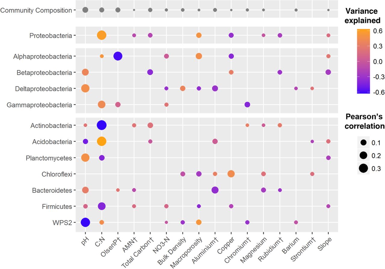 Open image in new tab
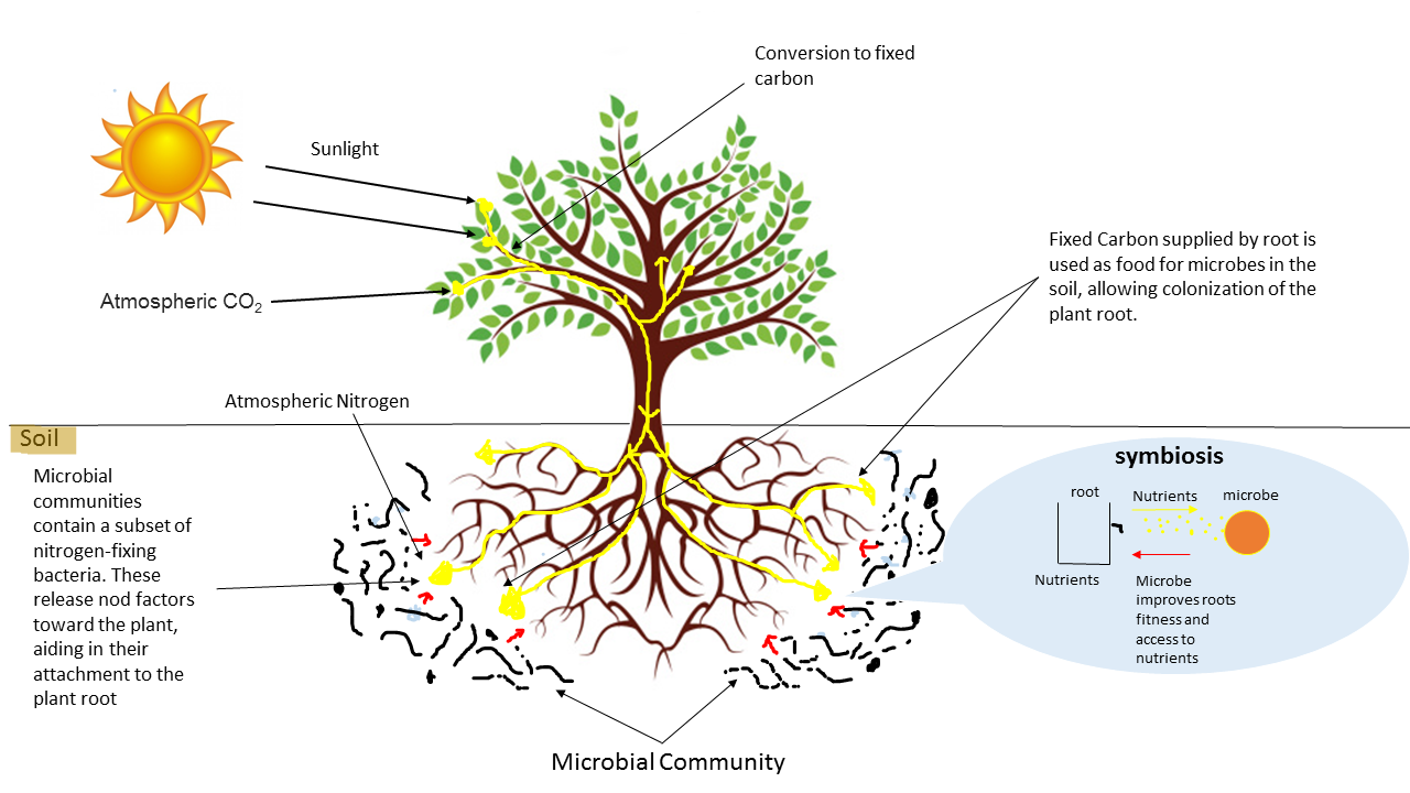
On the other hand, many species of microorganisms establish complex symbiotic relationships with plant organisms. The fraction of the substrate that is directly influenced by root secretions and associated microorganism is known as rhizosphere. Thus, for example, bacteria of the genus Bacillus, Pseudomonas or Burkholderia appear associated with the plant roots, protecting them from pathogenic microorganisms.
 Open image in new tab
In this tutorial, we will use sequencing data obtained through the MinION sequencer (Oxford Nanopore Technologies) with two objectives: 1) evaluate the health status of soil samples and 2) study how microbial populations are modified by their interaction with plant roots. This example was inspired by Brown et al. 2017.
AgendaIn this tutorial, we will cover:
Background on data
Next, we will introduce some details about the datasets that we are going to use to perform the analysis.
The datasets
In this example, we will use a dataset originally hosted in the NCBI SRA database, with the accession number SRP194577. To obtain the samples, the DNA was extracted using the Zymo Research Kit, followed by PCR amplification of 16S rRNA genes. Sequencing was carried out on a Nanopore Minion device. We are going to use four datasets, corresponding to two experimental conditions:
- Soil:
- Surface sample (0-5 cm):
bulk_top.fastq.gz - Deep sample (10-15 cm):
bulk_bottom.fastq.gz
- Surface sample (0-5 cm):
- Rhizosphere:
- Surface sample (0-5 cm):
rhizosphere_top.fastq.gz - Deep sample (10-15 cm):
rhizosphere_bottom.fastq.gz
- Surface sample (0-5 cm):
QuestionWhy do we sequence the 16S rRNA genes for analyzing microbial communities?
There are several reasons to use these genes as taxonomic markers. First, they are constituent parts of ribosomes, a piece of highly-conserved biological machinery, which makes them universally distributed. On the other hand, these genes present regions with varying degrees of sequence variability, which allows them to be used as a species-specific signature.
Get data
Hands On: Data upload
- Create a new history for this tutorial
Import the files from Zenodo:
- Open the file galaxy-upload upload menu
- Click on Collection tab
- Click of the Paste/Fetch button
Paste the Zenodo links and press Start and Build
https://zenodo.org/record/4274812/files/bulk_bottom.fastq.gz https://zenodo.org/record/4274812/files/bulk_top.fastq.gz https://zenodo.org/record/4274812/files/rhizosphere_bottom.fastq.gz https://zenodo.org/record/4274812/files/rhizosphere_top.fastq.gz- Assign a name to the new collection:
soil collection
- Copy the link location
Click galaxy-upload Upload at the top of the activity panel
- Select galaxy-wf-edit Paste/Fetch Data
Paste the link(s) into the text field
Press Start
- Close the window
As an alternative to uploading the data from a URL or your computer, the files may also have been made available from a shared data library:
- Go into Libraries (left panel)
- Navigate to the correct folder as indicated by your instructor.
- On most Galaxies tutorial data will be provided in a folder named GTN - Material –> Topic Name -> Tutorial Name.
- Select the desired files
- Click on Add to History galaxy-dropdown near the top and select as Datasets from the dropdown menu
In the pop-up window, choose
- “Select history”: the history you want to import the data to (or create a new one)
- Click on Import

Assess datasets quality
Before starting to work on our datasets, it is necessary to assess their quality. This is an essential step if we aim to obtain a meaningful downstream analysis.
FASTQ format is a text-based format for storing both a biological sequence and its corresponding quality scores. Both the sequence letter and the quality score are encoded with a single ASCII character for brevity. You can find more info in the Wikipedia article.
Quality control using FastQC and MultiQC
FastQC is one of the most widely used tools to check the quality of the samples generated by High Throughput Sequencing (HTS) technologies.
Hands On: Quality check
- FastQC ( Galaxy version 0.72+galaxy1) with the following parameters:
- param-collection “Dataset collection”:
soil collection- Rename the outputs as
FastQC unprocessed: RawandFastQC unprocessed: Web- MultiQC ( Galaxy version 1.8+galaxy1) with the following parameters:
- In “Results”:
- “Which tool was used generate logs?”:
FastQCparam-collection “Dataset collection”:
FastQC unprocessed: Raw- Click on the galaxy-eye (eye) icon and inspect the generated HTML file
FastQC provides information on various parameters, such as the range of quality values across all bases at each position. MultiQC allows summarizing the output of different outputs from FastQC.
 Open image in new tab
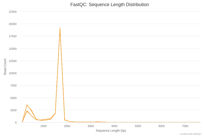
In the first place, we are going to analyse the sequence length distribution of the different datasets.
Question
- Can you explain the sequence length distribution plot?
The main peak, around 1700 bp, corresponds approximately to the length of the gene coding for 16S rRNA. There is also a secondary peak around 200 bp, which may be due to truncated amplifications, or as a result of non-specific hybridization of primers used for PCR.
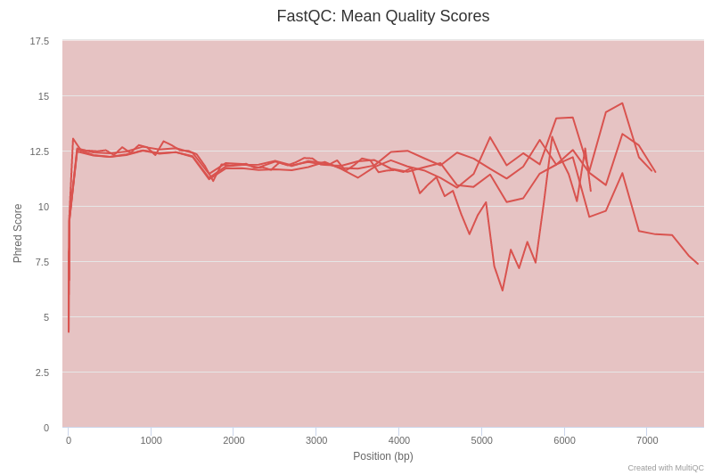 Open image in new tab
If we examine figure 3, we can see that up to 3000 bp the quality of our sequencing data is around a Phred score of 12, which is a relatively low value compared to other sequencing technologies. This is explained because Nanopore reads poses high error rates in the basecalled reads (10% as compared to 1% for Illumina). However, Nanopore sequencing generates very long reads (in theory only limited by the mechanisms of extraction of the genetic material), enabling the sequencing of the complete 16S rRNA gene, which makes it possible to identify bacterial taxa at higher resolution.
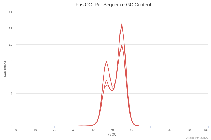 Open image in new tab
Let’s have a look at figure 4, which shows the content of the GC by sequence.
QuestionWhat can cause GC content to show a bimodal peak?
There are several possible causes for the presence of twin peaks in the GC content. One possible explanation is the presence of adapters in the sequence. Another possible cause is some kind of contamination, such as chimeras.
CommentFor more information on the topic, please see the quality control tutorial.
Improve the dataset quality
In order to improve the quality of our data, we will use two tools presented above, porechop and fastp.
Adapter and chimera removal with porechop
Nanopore sequencing technology requires to ligate adapters to both ends of genomic material to facilitate the strand capture and loading of a processive enzyme at the 5’end, boosting the effectiveness of the sequencing process. Adapter sequences should be removed because they can interfere with aligment of reads to 16S rRNA gene reference database, for which we will use the porechop tool (Wick 2017).
CommentIf you are interested in Nanopore sequecing technology, you can find more information in Jain et al. 2016.
On the other hand, chimeric sequences are considered a contaminant and should be removed because they can result in artificial inflation of the microbial diversity. With Porechop you can eliminate them.
Hands On: Remove adapters with porechop
- Porechop ( Galaxy version 0.2.3) with the following parameters:
- “Input FASTA/FASTQ”: param-collection
soil collection- “Output format for the reads”:
fastq- Rename the output as
soil collection trimmed
Filter sequences with fastp
To increase the specificity of the analysis, we will select the reads with lengths between 1000 bp and 2000 bp, which are more informative from a taxonomic point of view, because they include both preserved and hypervariable regions of the 16S rRNA gene. In addition, sequences will be filtered on a minimum average read quality score of 9, according to the recommendations from Nygaard et al. 2020. This stage will be carried out through the use of fastp (Chen et al. 2018), an open-source tool designed to process FASTQ files.
Hands On: Filter sequence with fastp
- fastp ( Galaxy version 0.20.1+galaxy0) with the following parameters:
- “Single-end or paired reads”:
Single-end- param-collection “Dataset collection”:
soil collection trimmed
- In “Adapter Trimming Options”:
- “Disable adapter trimming”:
Yes- In “Filter Options”:
- In “Quality filtering options”:
- “Qualified quality phred”:
9- In “Length filtering options”:
- “Length required”:
1000- “Maximum length”:
2000- In “Read Modification Options”:
- “PolyG tail trimming”:
Disable polyG tail trimming- Rename the output as
soil collection processed
Re-evaluate datasets quality
After processing the sequences, we are going to analyze them again using FastQC and MultiQC to see if we have managed to correct the anomalies that we had detected.
Hands On: Quality check
- FastQC ( Galaxy version 0.72+galaxy1) with the following parameters:
- param-collection “Dataset collection”:
soil collection processed- Rename the outputs as
FastQC processed: RawandFastQC processed: Web- MultiQC ( Galaxy version 1.8+galaxy1) with the following parameters:
- In “Results”:
- “Which tool was used generate logs?”:
FastQCparam-collection “Dataset collection”:
FastQC processed: Raw- Click on the galaxy-eye (eye) icon and inspect the generated HTML file
We can verify that after processing the samples, the GC content presents a unimodal distribution, which indicates that the anomalies in the sequences have been successfully eliminated (Figure 6).
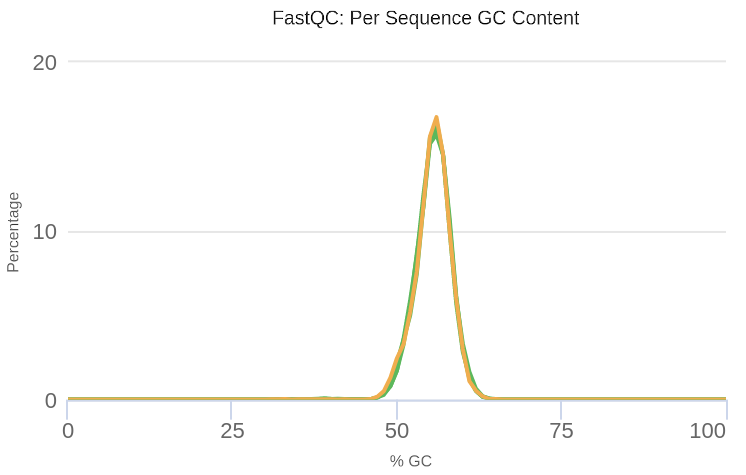 Open image in new tab
Assign taxonomic classifications
One of the key steps in metagenomic data analysis is to identify the taxon to which the individual reads belong. Taxonomic classification tools are based on microbial genome databases to identify the origin of each sequence.
Taxonomic classification with Kraken2
To perform the taxonomic classification we will use Kraken2 (Wood et al. 2019). This tool uses the minimizer method to sample the k-mers (all the read’s subsequences of length k) in a deterministic fashion in order to reduce memory constumption and processing time. In addition, it masks low-complexity sequences from reference sequences by using dustmasker.
In the \(k\)-mer approach for taxonomy classification, we use a database containing DNA sequences of genomes whose taxonomy we already know. On a computer, the genome sequences are broken into short pieces of length \(k\) (called \(k\)-mers), usually 30bp.
Kraken examines the \(k\)-mers within the query sequence, searches for them in the database, looks for where these are placed within the taxonomy tree inside the database, makes the classification with the most probable position, then maps \(k\)-mers to the lowest common ancestor (LCA) of all genomes known to contain the given \(k\)-mer.
Kraken2 uses a compact hash table, a probabilistic data structure that allows for faster queries and lower memory requirements. It applies a spaced seed mask of s spaces to the minimizer and calculates a compact hash code, which is then used as a search query in its compact hash table; the lowest common ancestor (LCA) taxon associated with the compact hash code is then assigned to the k-mer.
You can find more information about the Kraken2 algorithm in the paper Improved metagenomic analysis with Kraken 2.
 of the genomes that contain that k-mer in the database. The taxa associated with the sequence's k-mers, as well as the taxa's ancestors, form a pruned subtree of the general taxonomy tree, which is used for classification. In the classification tree, each node has a weight equal to the number of k-mers in the sequence associated with the node's taxon. Each root-to-leaf (RTL) path in the classification tree is scored by adding all weights in the path, and the maximal RTL path in the classification tree is the classification path (nodes highlighted in yellow). The leaf of this classification path (the orange, leftmost leaf in the classification tree) is the classification used for the query sequence. Source: <span class=\"citation\"><a href=\"#Wood2014\">Wood and Salzberg 2014</a></span>")
For this tutorial, we will use the SILVA database (Quast et al. 2012). It includes over 3.2 million 16S rRNA sequences from the Bacteria, Archaea and Eukaryota domains.
Hands On: Assign taxonomic labels with Kraken2
- Kraken2 ( Galaxy version 2.0.8_beta+galaxy0) with the following parameters:
- “Single or paired reads”:
Single- param-collection “Dataset collection”:
soil collection processed- “Print scientific names instead of just taxids”:
Yes- “Confidence”:
0.1- In “Create Report”:
- “Print a report with aggregrate counts/clade to file”:
Yes- “Format report output like Kraken 1’s kraken-mpa-report”:
Yes- “Select a Kraken2 database”:
Silva (Created: 2020-06-24T164526Z, kmer-len=35, minimizer-len=31, minimizer-spaces=6)CommentA confidence score of 0.1 means that at least 10% of the k-mers should match entries in the database. This value can be reduced if a less restrictive taxonomic assignation is desired.
Analyze taxonomic assigment
Once we have assigned the corresponding taxa to each sequence, the next step is to properly visualize the data, for which we will use the Krona pie chart tool (Ondov et al. 2011). But before that, we need to adjust the format of the data output from Kraken2.
Hands On: Adjust dataset format
- Reverse ( Galaxy version 1.1.0) with the following parameters:
- param-collection “Dataset collection”:
Report: Kraken2 on collection- Replace Text ( Galaxy version 1.1.2) with the following parameters:
- param-collection “Dataset collection”:
Reverse on collection- In “Replacement”:
- param-repeat “Insert Replacement”
- “Find pattern”:
\|- “Replace with”:
\t- Remove beginning with the following parameters:
- param-collection “Dataset collection”:
Replace Text on collection
Visualize the taxonomical classification with Krona
Krona allows hierarchical data to be explored with zooming, multi-layered pie charts. With this tool, we can easily visualize the composition of the bacterial communities and compare how the populations of microorganisms are modified according to the conditions of the environment.
Hands On: Visualize metagenomics analysis results
- Krona pie chart ( Galaxy version 2.7.1) with the following parameters:
- “What is the type of your input data”:
Tabular- param-collection “Dataset collection”:
Remove beginning on collection- “Provide a name for the basal rank”:
Bacteria
Let’s take a look at the result. Using the search bar we can check if certain taxa are present.
Question
- What can we say about the health status of the soil samples?
- Are there significant differences in the bacterial population structure between soil samples and rhizosphere samples?
- The low presence of Alphaproteobacteria (including members of the order Rhizobiales), as well as the abundance of Bacteroidetes and Gammaproteobacteria, suggest that the soil is highly exposed to phosphorus. This mineral is strongly associated with the anthropogenic activity as it is an important component of agrochemicals.
- We can observe that there are important differences in the structure of the bacterial populations between the soil and rhizosphere samples. Particularly significant is the increase in phylum Planctomycetes, which are usually abundant in the rhizosphere.
Conclusion
In this tutorial we used MinION Nanopore sequencing data to study the health status of soil samples and the structure of bacterial populations. The results indicate that the soil suffers some degree of erosion as a result of their exposure to agrochemicals. We have also been able to study how the composition of microbial communities is modified in presence of plant organisms.
You've Finished the Tutorial
Key points
We learned to use MinION Nanopore data for analyzing the health status of the soil
We preprocessed Nanopore sequences in order to improve their quality
Frequently Asked Questions
Have questions about this tutorial? Have a look at the available FAQ pages and support channelsUseful literature
Further information, including links to documentation and original publications, regarding the tools, analysis techniques and the interpretation of results described in this tutorial can be found here.
References
- Fierer, N., and R. B. Jackson, 2006 The diversity and biogeography of soil bacterial communities. Proceedings of the National Academy of Sciences 103: 626–631. 10.1073/pnas.0507535103
- Ondov, B. D., N. H. Bergman, and A. M. Phillippy, 2011 Interactive metagenomic visualization in a Web browser. BMC Bioinformatics 12: 10.1186/1471-2105-12-385
- Quast, C., E. Pruesse, P. Yilmaz, J. Gerken, T. Schweer et al., 2012 The SILVA ribosomal RNA gene database project: improved data processing and web-based tools. Nucleic Acids Research 41: D590–D596. 10.1093/nar/gks1219
- Wood, D. E., and S. L. Salzberg, 2014 Kraken: ultrafast metagenomic sequence classification using exact alignments. Genome Biology 15: R46. 10.1186/gb-2014-15-3-r46
- Hermans, S. M., H. L. Buckley, B. S. Case, F. Curran-Cournane, M. Taylor et al., 2016 Bacteria as Emerging Indicators of Soil Condition (F. E. Loeffler, Ed.). Applied and Environmental Microbiology 83: 10.1128/aem.02826-16
- Jain, M., H. E. Olsen, B. Paten, and M. Akeson, 2016 The Oxford Nanopore MinION: delivery of nanopore sequencing to the genomics community. Genome Biology 17: 10.1186/s13059-016-1103-0
- Brown, B. L., M. Watson, S. S. Minot, M. C. Rivera, and R. B. Franklin, 2017 MinION™ nanopore sequencing of environmental metagenomes: a synthetic approach. GigaScience 6: 10.1093/gigascience/gix007
- Wick, R., 2017 Porechop. GitHub. https://github.com/rrwick/Porechop
- Chen, S., Y. Zhou, Y. Chen, and J. Gu, 2018 fastp: an ultra-fast all-in-one FASTQ preprocessor. 10.1101/274100
- Wood, D. E., J. Lu, and B. Langmead, 2019 Improved metagenomic analysis with Kraken 2. Genome Biology 20: 10.1186/s13059-019-1891-0
- Nygaard, A. B., H. S. Tunsjø, R. Meisal, and C. Charnock, 2020 A preliminary study on the potential of Nanopore MinION and Illumina MiSeq 16S rRNA gene sequencing to characterize building-dust microbiomes. Scientific Reports 10: 3209. 10.1038/s41598-020-59771-0
Feedback
Did you use this material as an instructor? Feel free to give us feedback on how it went.
Did you use this material as a learner or student? Click the form below to leave feedback.

Citing this Tutorial
- Cristóbal Gallardo, 16S Microbial analysis with Nanopore data (Galaxy Training Materials). https://training.galaxyproject.org/training-material/topics/microbiome/tutorials/nanopore-16S-metagenomics/tutorial.html Online; accessed TODAY
- Hiltemann, Saskia, Rasche, Helena et al., 2023 Galaxy Training: A Powerful Framework for Teaching! PLOS Computational Biology 10.1371/journal.pcbi.1010752
- Batut et al., 2018 Community-Driven Data Analysis Training for Biology Cell Systems 10.1016/j.cels.2018.05.012
Congratulations on successfully completing this tutorial!@misc{microbiome-nanopore-16S-metagenomics, author = "Cristóbal Gallardo", title = "16S Microbial analysis with Nanopore data (Galaxy Training Materials)", year = "", month = "", day = "", url = "\url{https://training.galaxyproject.org/training-material/topics/microbiome/tutorials/nanopore-16S-metagenomics/tutorial.html}", note = "[Online; accessed TODAY]" } @article{Hiltemann_2023, doi = {10.1371/journal.pcbi.1010752}, url = {https://doi.org/10.1371%2Fjournal.pcbi.1010752}, year = 2023, month = {jan}, publisher = {Public Library of Science ({PLoS})}, volume = {19}, number = {1}, pages = {e1010752}, author = {Saskia Hiltemann and Helena Rasche and Simon Gladman and Hans-Rudolf Hotz and Delphine Larivi{\`{e}}re and Daniel Blankenberg and Pratik D. Jagtap and Thomas Wollmann and Anthony Bretaudeau and Nadia Gou{\'{e}} and Timothy J. Griffin and Coline Royaux and Yvan Le Bras and Subina Mehta and Anna Syme and Frederik Coppens and Bert Droesbeke and Nicola Soranzo and Wendi Bacon and Fotis Psomopoulos and Crist{\'{o}}bal Gallardo-Alba and John Davis and Melanie Christine Föll and Matthias Fahrner and Maria A. Doyle and Beatriz Serrano-Solano and Anne Claire Fouilloux and Peter van Heusden and Wolfgang Maier and Dave Clements and Florian Heyl and Björn Grüning and B{\'{e}}r{\'{e}}nice Batut and}, editor = {Francis Ouellette}, title = {Galaxy Training: A powerful framework for teaching!}, journal = {PLoS Comput Biol} }
You can use Ephemeris's
shed-tools installcommand to install the tools used in this tutorial.shed-tools install [-g GALAXY] [-a API_KEY] -t <(curl https://training.galaxyproject.org/training-material/api/topics/microbiome/tutorials/nanopore-16S-metagenomics/tutorial.json | jq .admin_install_yaml -r)Alternatively you can copy and paste the following YAML
---
install_tool_dependencies: true
install_repository_dependencies: true
install_resolver_dependencies: true
tools:
- name: text_processing
  owner: bgruening
  revisions: d698c222f354
  tool_panel_section_label: Text Manipulation
  tool_shed_url: https://toolshed.g2.bx.psu.edu/
- name: taxonomy_krona_chart
  owner: crs4
  revisions: 1334cb4c6b68
  tool_panel_section_label: Metagenomic Analysis
  tool_shed_url: https://toolshed.g2.bx.psu.edu/
- name: fastqc
  owner: devteam
  revisions: e7b2202befea
  tool_panel_section_label: FASTA/FASTQ
  tool_shed_url: https://toolshed.g2.bx.psu.edu/
- name: datamash_reverse
  owner: iuc
  revisions: 0f1724dd59d2
  tool_panel_section_label: Join, Subtract and Group
  tool_shed_url: https://toolshed.g2.bx.psu.edu/
- name: fastp
  owner: iuc
  revisions: dbf9c561ef29
  tool_panel_section_label: FASTA/FASTQ
  tool_shed_url: https://toolshed.g2.bx.psu.edu/
- name: kraken2
  owner: iuc
  revisions: 328c607150ff
  tool_panel_section_label: Metagenomic Analysis
  tool_shed_url: https://toolshed.g2.bx.psu.edu/
- name: multiqc
  owner: iuc
  revisions: 5e33b465d8d5
  tool_panel_section_label: Quality Control
  tool_shed_url: https://toolshed.g2.bx.psu.edu/
- name: porechop
  owner: iuc
  revisions: 93d623d9979c
  tool_panel_section_label: Nanopore
  tool_shed_url: https://toolshed.g2.bx.psu.edu/