Advances in sequencing technologies over the last few decades have revolutionized the field of genomics, allowing for a reduction in both the time and resources required to perform de novo genome assembly. Until recently, second-generation sequencing technologies (also known as next generation sequencing (NGS)) produced highly accurate but short (up to 800bp) reads. These read lengths were not long enough to cope with the difficulties associated with repetitive regions. Today, so-called third-generation sequencing (TGS) technologies, also known as single-molecule real-time (SMRT) sequencing, have become dominant in de novo assembly of large genomes. TGS can use native DNA without amplification, reducing sequencing error and bias (Hon et al. 2020, Giani et al. 2020). In 2020, PacBio introduced high fidelity (HiFi) sequencing, which produces reads 10-25 kbp in length with a minimum accuracy of 99% (Q20). In this tutorial, you will use HiFi reads in combination with data from additional sequencing technologies to generate a high-quality genome assembly.
Deciphering the structural organization of complex vertebrate genomes is currently one of the largest challenges in genomics (Frenkel et al. 2012). Despite the significant progress made in recent years, a key question remains: what combination of data and tools can produce the highest quality assembly? In order to adequately answer this question, it is necessary to analyse two of the main factors that determine the difficulty of genome assembly processes: repetitive content and heterozygosity.
Repetitive elements can be grouped into two categories: interspersed repeats, such as transposable elements (TE) that occur at multiple loci throughout the genome, and tandem repeats (TR) that occur at a single locus (Tørresen et al. 2019). Repetitive elements are an important component of eukaryotic genomes, constituting over a third of the genome in the case of mammals (Sotero-Caio et al. 2017, Chalopin et al. 2015). In the case of tandem repeats, various estimates suggest that they are present in at least one third of human protein sequences (Marcotte et al. 1999). TE content is among the main factors contributing to the lack of continuity in the reconstruction of genomes, especially in the case of large ones, as TE content is highly correlated with genome size (Sotero-Caio et al. 2017). On the other hand, TR usually lead to local genome assembly collapse, especially when their length is close to that of the reads (Tørresen et al. 2019).
Heterozygosity is also an important factor impacting genome assembly. Haplotype phasing, the identification of alleles that are co-located on the same chromosome, has become a fundamental problem in heterozygous and polyploid genome assemblies (Zhang et al. 2020). When no reference sequence is available, the state-of-the-art strategy consists of constructing a string graph with vertices representing reads and edges representing consistent overlaps. In this kind of graph, after transitive reduction, heterozygous alleles in the string graph are represented by bubbles. When combined with all-versus-all chromatin conformation capture (Hi-C) data, this approach allows complete diploid reconstruction (Angel et al. 2018, Zhang et al. 2020, Dida and Yi 2021).
The Genome 10K consortium (G10K) launched the Vertebrate Genome Project (Vertebrate Genomes Project (VGP)), whose goal is generating high-quality, near-error-free, gap-free, chromosome-level, haplotype-phased, annotated reference genome assemblies for every vertebrate species (Rhie et al. 2020). This tutorial will guide you step by step to assemble a high-quality genome using the VGP assembly pipeline, including multiple Quality Control (QC) evaluations.
Warning: Your results may differ!
Some of your results may slightly differ from the results shown in this tutorial, depending on the versions of the tools used, since algorithms can change between versions.
Before getting into the thick of things, let’s go over some terms you will often hear when learning about genome assembly. These concepts will be used often throughout this tutorial as well, so please refer to this section as necessary to help your understanding.
Pseudohaplotype assembly: A genome assembly that consists of long-phased haplotype blocks separated by regions where the haplotype cannot be distinguished (often homozygous regions). This can result in “switch errors”, when the parental haplotypes alternate along the same sequence. These types of assemblies are usually represented by a primary assembly and an alternate assembly. (This definition is largely taken from the NCBI’s Genome Assembly Model.)
Primary assembly: The primary assembly is traditionally the more complete representation of an individual’s genome and consists of homozygous regions and one set of loci for heterozygous regions. Because the primary assembly contains both homo- and heterozygous regions, it is more complete than the alternate assambly which often reports only the other allele for heterozygous regions. Thus, the primary assembly is usually what one would use for downstream analyses.
Alternate assembly: The alternate assembly consists of the alternate alleles not represented in the primary assembly (heterozygous loci from the other haplotype). These types of sequences are often referred to as haplotigs. Traditionally, the alternate assembly is less complete compared to the primary assembly since homozygous regions are not represented.
Phasing: Phasing aims to partition the contigs for an individual according to the haplotype they are derived from. When parental data is available, this is done by identifying parental alleles using read data from the parents. Locally, this is achieved using linkage information in long read datasets. Recent approaches have managed to phase using long-range Hi-C linkage information from the same individual (Cheng et al. 2021).
Assembly graph: A representation of the genome inferred from sequencing reads. Sequencing captures the genome as many fragmented pieces, instead of whole entire chromosomes at once (we eagerly await the day when this statement will be outdated!). The start of the assembly process pieces together these genome fragments to generate an assembly graph, which is a representation of the sequences and their overlaps. Visualizing assembly graphs can show where homozygous regions branch off into alternate paths on different haplotypes.
Unitig: Usually the smallest unit of an assembly graph, consistent with all the available sequencing data. A unitig is often constructed from an unambiguous path in the assembly graph where all the vertices have exactly one incoming and one outgoing edge, except the first vertex can have any number of incoming edges, while the last vertex can have any number of outgoing edges (Rahman and Medvedev 2022). In other words, the internal vertices in the unitig path can only be walked one way, so unitigs represent a path of confident sequence. In the assembly graph, unitig nodes can then have overlap edges with other unitigs.
Contig: A contiguous (i.e., gapless) sequence in an assembly, usually inferred algorithmically from the unitig graph.
False duplications: Assembly errors that result in one region of the genome being represented twice in the same assembly as two separate regions. Not to be confused with optical or technical duplicates from PCR from short-read sequencing. False duplications can further be classified as either haplotypic duplications or overlaps.
Haplotypic duplication can happen when a region that is heterozygous in the individual has the two haplotypes showing enough divergence that the assembler fails to interpret them as homologous. For example, say an individual is heterozygous in the region Chr1[1:100] and has Haplotype A from their mother and Haplotype B from their father; a false duplication can arise when the haplotypes are not recognized as being from the same region, and the assembler ends up placing both haplotypes in the same assembly, resulting in Chr1[1:100] being represented twice in one assembly. Ideally, a properly phased assembly would have Haplotype A in one assembly, e.g., the primary, while Haplotype B is in the alternate.
False duplications via overlaps result from unresolved overlaps in the assembly graph. In this case, two different contigs end up representing the same sequence, effectively duplicating it. Overlaps happen when a branching point in an assembly graph is resolved such that the contig before the vertex and a contig after the vertex share the same overlapping sequence.
Figure 1: Schematic of types of false duplication. Image adapted from Rhie et al. 2020.
Purging: Purging aims to remove false duplications, collapsed repeats, and very low support/coverage regions from an assembly. When performed on a primary assembly, the haplotigs are removed from the primary and typically placed in the alternate assembly.
Scaffold: A scaffold refers to one or more contigs separated by gap (unknown) sequence. Scaffolds are usually generated with the aid of additional information, such as Bionano optical maps, linked reads, Hi-C chromatin information, etc. The regions between contigs are usually of unknown sequence, thus they are represented by sequences of N’s. Gap length in the sequence can be sized or arbitrary, depending on the technology used for scaffolding (e.g., optical maps can introduce sized gaps, while scaffolding software using Hi-C information usually uses an arbitrary number of N’s, such as 500 or 200).
For more about the specific scaffolding technologies used in the VGP pipeline (currently Bionano optical maps and Hi-C chromatin conformation data), please refer to those specific sections within this tutorial.
HiFi reads: PacBio HiFi reads are the focus of this tutorial. First described in 2019, they have revolutionized genome assembly by combining long (about 10-20 kbp) read lengths with high accuracy (>Q20) typically associated with short-read sequencing (Wenger et al. 2019). These higher read lengths enable HiFi reads to traverse some repeat regions that are problematic to assemble with short reads.
Ultra-long reads: Ultra-long reads are typically defined as reads of over 100 kbp, and are usually generated using Oxford Nanopore Technology. Read quality is often lower than HiFi or Illumina (i.e., have a higher error rate), but they are often significantly longer than any other current sequencing technology, and can help assembly algorithms walk complex repeat regions in the assembly graphs.
Manual curation: This term refers to manually evaluating and manipulating an assembly based on the raw supporting evidence (e.g., using Hi-C contact map information). The user takes into account the original sequencing data to resolve potential misassemblies and missed joins.
Misassembly: Misassemblies are a type of assembly error that usually refers to any structural error in the genome reconstruction, e.g., sequences that are not adjacent in the genome being placed next to each other in the sequence. Misassemblies can be potentially identified and remedied by manual curation.
Missed join: A missed join happens when two sequences are adjacent to each other in the genome but are not represented contiguously in the final sequence. Missed joins can be identified and remedied in manual curation with Hi-C data.
Telomere-to-telomere assembly: Often abbreviated as “T2T”, this term refers to an assembly where each chromosome is completely gapless from telomere to telomere. The term usually refers to the recently completed CHM13 human genome (Nurk et al. 2022), though there is an increasing number of efforts to generate T2T genomes for other species.
VGP assembly pipeline overview
The VGP assembly pipeline has a modular organization, consisting of ten workflows (Fig. 1). It can used with the following types of input data:
Properly phased with even more improved contiguity
H
In this table, HiFi and Hi-C refer to HiFi and Hi-C data derived from the individual whose genome is being assembled. This tutorial assumes you are assembling the genome of one individual; there are special considerations necessary for pooled data that are not covered in this tutorial. (Note: you can use Hi-C data from another individual of the same species to scaffold, but you cannot use that data to phase the contigs in hifiasm.) Parental data is high-coverage whole genome resequencing data derived from the parents of the individual being assembled, and is the key component of trio-based genome assembly. Each combination of input datasets is demonstrated in Fig. 2 by an analysis trajectory: a combination of workflows designed for generating the best assembly given a particular combination of inputs. These trajectories are listed in the table above and shown in the figure below.
Figure 2: Eight analysis trajectories are possible depending on the combination of input data. A decision on whether or not to invoke Workflow 6 is based on the analysis of QC output of workflows 3, 4, or 5. Thicker lines connecting Workflows 7, 8, and 9 represent the fact that these workflows are invoked separately for each phased assembly (once for maternal and once for paternal).
The stages of genome assembly in the VGP-Galaxy pipeline are generally:
K-mer profiling: the generation of k-mer profiles of the raw reads to estimate genome size, heterozygosity, repetitiveness, and error rate. This is useful for getting an idea of the genome that lies within your reads, and is also useful for necessary for parameterizing downstream workflows. The generation of k-mer counts can be done from HiFi data only (Workflow 1), or include data from parental reads for trio-based phasing (Workflow 2), if one wants to generate k-mer spectra for the individual’s parents, as well.
Contig assembly: In addition to using only HiFi reads (Workflow 3), the contig building (contiging) step can leverage Hi-C (Workflow 4) or parental read data (Workflow 5) to produce fully-phased haplotypes (hap1/hap2 or parental/maternal assigned haplotypes), using hifiasm. The contiging workflows also produce a number of critical quality control (QC) metrics such as k-mer multiplicity profiles. Inspection of these profiles provides information to decide whether the third stage—purging of false duplication—is required.
(Optional) Purging: Purging duplicates (Workflow 6) using purge_dups identifies and resolves haplotype-specific assembly segments incorrectly labeled as primary contigs, as well as heterozygous contig overlaps. This increases contiguity and the quality of the final assembly. The purging stage is generally unnecessary for trio data, as haplotype resolution is attained using set operations done on parental k-mers.
Scaffolding: Scaffolding produces chromosome-level scaffolds using information provided by Bionano (Workflow 7, with Bionano Solve (optional)) and Hi-C (Workflow 8, with YaHS algorithms).
Decontamination: A final step of decontamination (Workflow 9) removes non-target sequences (e.g., contamination as well as mitochondrial sequences) from the scaffolded assembly. A separate workflow (WF0) is used for mitochondrial assembly.
Comment: A note on data quality
For diploids, we suggest at least 30✕ PacBio HiFi coverage & around 60✕ Hi-C coverage, and up to 60✕ HiFi coverage to accurately assemble highly repetitive regions.
This training has been organized into four main sections: genome profile analysis, assembly of HiFi reads with hifiasm, scaffolding with Bionano optical maps, and scaffolding with Hi-C data. Additionally, the assembly with hifiasm section has two possible paths in this tutorial: solo contiging or solo w/HiC contiging.
Throughout this tutorial, there will be detail boxes with additional background information on the science behind the sequencing technologies and software we use in the pipeline. These boxes are minimized by default, but please expand them to learn more about the data we utilize in this pipeline.
Get data
In order to reduce computation time, we will assemble samples from the yeast Saccharomyces cerevisiae S288C, a widely used laboratory strain isolated in the 1950s by Robert Mortimer. Using S. cerevisae, one of the most intensively studied eukaryotic model organisms, has the additional advantage of allowing us to evaluate the final result of our assembly with great precision. For this tutorial, we generated a set of synthetic HiFi reads corresponding to a theoretical diploid genome.
The synthetic HiFi reads were generated by using the S288C assembly as reference genome. With this objective we used HIsim, a HiFi shotgun simulator. The commands used are detailed below:
The selected mutation rate was 2%. Note that HIsim generates the synthetic reads in FASTA format. This is perfectly fine for illustrating the workflow, but you should be aware that usually you will work with HiFi reads in FASTQ format.
The first step is to get the datasets from Zenodo. Specifically, we will be uploading two datasets:
A set of PacBio HiFi reads in fasta format. Please note that your HiFi reads received from a sequencing center will usually be fastqsanger.gz format, but the dataset used in this tutorial has been converted to fasta for space.
A set of Illumina Hi-C reads in fastqsanger.gz format.
Uploading fasta datasets from Zenodo
The following two steps demonstrate how to upload three PacBio HiFi datasets into your Galaxy history.
Hands On: Uploading FASTA datasets from Zenodo
Create a new history for this tutorial
To create a new history simply click the new-history icon at the top of the history panel:
Copy the following URLs into the clipboard.
you can do this by clicking on copy button in the right upper corner of the box below. It will appear if you mouse over the box.
Click galaxy-uploadUpload at the top of the activity panel
Select galaxy-wf-editPaste/Fetch Data
Paste the link(s) into the text field
Change Type (set all): from “Auto-detect” to fasta
Press Start
Close the window
Uploading fasta or fasta.gz datasets via URL.
Uploading fastqsanger.gz datasets from Zenodo
Illumina Hi-C data is uploaded in essentially the same way as shown in the following two steps.
Warning: DANGER: Make sure you choose the correct format!
When selecting datatype in “Type (set all)” drop-down, make sure you select fastaqsanger or fastqsanger.gz BUT NOT fastqcssanger or anything else!
Hands On: Uploading fastqsanger.gz datasets from Zenodo
Copy the following URLs into the clipboard. You can do this by clicking on copy button in the right upper corner of the box below. It will appear if you mouse over the box.
Upload datasets into Galaxy and set the datatype to fastqsanger.gz
Copy the link location
Click galaxy-uploadUpload at the top of the activity panel
Select galaxy-wf-editPaste/Fetch Data
Paste the link(s) into the text field
Change Type (set all): from “Auto-detect” to fastqsanger.gz
Press Start
Close the window
Uploading fastqsanger or fastqsanger.gz datasets via URL.
Click on Upload Data on the top of the left panel:
Click on Paste/Fetch:
Paste URL into text box that would appear:
Set Type (set all) to fastqsanger or, if your data is compressed as in URLs above (they have .gz extensions), to fastqsanger.gz
:
Warning: Danger: Make sure you choose corect format!
When selecting datatype in “Type (set all)” dropdown, make sure you select fastaqsanger or fastqsanger.gz BUT NOT fastqcssanger or anything else!
Rename the datasets as follow:
Rename SRR7126301_1.fastq.gz as Hi-C_dataset_F. It contains the forward reads.
Rename SRR7126301_2.fastq.gz as Hi-C_dataset_R. It contains the reverse reads.
Warning: These datasets are large!
Hi-C datasets are large. It will take some time (~15 min) for them to be fully uploaded. Please, be patient.
Organizing the data
If everything goes smoothly your history will look like shown in the figure below. The three HiFi fasta files are better represented as a collection: {collection}. Also, importantly, the workflow we will be using for the analysis of our data takes a collection as input (it does not access individual datasets). So let’s create a collection using steps outlined in the Tip tip “Creating a dataset collection”:
Click on galaxy-selectorSelect Items at the top of the history panel
Check all the datasets in your history you would like to include
Click n of N selected and choose Advanced Build List
You are in collection building wizard. Choose Flat List and click ‘Next’ button at the right bottom corner.
Double clcik on the file names to edit. For example, remove file extensions or common prefix/suffixes to cleanup the names.
Enter a name for your collection
Click Build to build your collection
Click on the checkmark icon at the top of your history again
The view of your history should transition from what is shown in the left pane below to what looks like the right pane:
Figure 3: History after uploading HiFi and HiC data (left). Creation of a list (collection) combines all HiFi datasets into a single history item called 'HiFi data' (right). See below for instructions on how to make this collection.
You can obviously upload your own datasets via URLs as illustrated above or from your own computer. In addition, you can upload data from a major repository called GenomeArk. GenomeArk is integrated directly into Galaxy Upload. To use GenomeArk follow the steps in the Tip tip below:
Open the file galaxy-uploadupload menu
Click on Choose remote files tab
Click on the Genome Ark button and then click on species
You can find the data by following this path: /species/${Genus}_${species}/${specimen_code}/genomic_data. Inside a given datatype directory (e.g.pacbio), select all the relevant files individually until all the desired files are highlighted and click the Ok button. Note that there may be multiple pages of files listed. Also note that you may not want every file listed.
HiFi reads preprocessing with cutadapt
Adapter trimming usually means trimming the adapter sequence off the ends of reads, which is where the adapter sequence is usually located in NGS reads. However, due to the nature of SMRT sequencing technology, adapters do not have a specific, predictable location in HiFi reads. Additionally, the reads containing adapter sequences could be of generally lower quality compared to the rest of the reads. Thus, we will use cutadapt not to trim, but to remove the entire read if a read is found to have an adapter inside of it.
PacBio HiFi reads rely on SMRT sequencing technology. SMRT is based on real-time imaging of fluorescently tagged nucleotides as they are added to a newly synthesized DNA strand. HiFi further uses multiple subreads from the same circular template to produce one highly accurate consensus sequence (fig. 2).
Figure 4: HiFi reads are produced by calling consensus from subreads generated by multiple passes of the enzyme around a circularized template. This results in a HiFi read that is both long and accurate.
This technology allows to generate long-read sequencing data with read lengths in the range of 10-25 kb and minimum read consensus accuracy greater than 99% (Q20).
Hands On: Primer removal with Cutadapt
Run Cutadapt ( Galaxy version 4.4+galaxy0) with the following parameters:
“Single-end or Paired-end reads?”: Single-end
param-collection“FASTQ/A file”: HiFi_collection
In “Read 1 Options”:
In “5’ or 3’ (Anywhere) Adapters”:
param-repeat“Insert 5’ or 3’ (Anywhere) Adapters”
“Source”: Enter custom sequence
“Enter custom 5’ or 3’ adapter name”: First adapter
“Enter custom 5’ or 3’ adapter sequence”: ATCTCTCTCAACAACAACAACGGAGGAGGAGGAAAAGAGAGAGAT
param-repeat“Insert 5’ or 3’ (Anywhere) Adapters”
“Source”: Enter custom sequence
“Enter custom 5’ or 3’ adapter name”: Second adapter
“Enter custom 5’ or 3’ adapter sequence”: ATCTCTCTCTTTTCCTCCTCCTCCGTTGTTGTTGTTGAGAGAGAT
In “Adapter Options”:
“Maximum error rate”: 0.1
“Minimum overlap length”: 35
“Look for adapters in the reverse complement”: Yes
In “Filter Options”:
“Discard Trimmed Reads”: Yes
Click on param-collectionDataset collection in front of the input parameter you want to supply the collection to.
Select the collection you want to use from the list
Rename the output file as HiFi_collection (trimmed).
Click on the galaxy-pencilpencil icon for the dataset to edit its attributes
In the central panel, change the Name field
Click the Save button
Genome profile analysis
Before starting a de novo genome assembly project, it is useful to collect metrics on the properties of the genome under consideration, such as the expected genome size, so that you know what to expect from your assembly. Traditionally, DNA flow cytometry was considered the golden standard for estimating the genome size. Nowadays, experimental methods have been replaced by computational approaches (Wang et al. 2020). One widely used genome profiling methods is based on the analysis of k-mer frequencies. It allows one to provide information not only about the genomic complexity, such as the genome size and levels of heterozygosity and repeat content, but also about the data quality.
K-mers are unique substrings of length k contained within a DNA sequence. For example, the DNA sequence TCGATCACA can be decomposed into five unique k-mers that have five bases long: TCGAT, CGATC, GATCA, ATCAC and TCACA. A sequence of length L will have L-k+1 k-mers. On the other hand, the number of possible k-mers can be calculated as nk, where n is the number of possible monomers and k is the k-mer size.
Bases
k-mer size
Total possible k-mers
4
1
4
4
2
16
4
3
64
4
…
…
4
10
1.048.576
Thus, the k-mer size is a key parameter, which must be large enough to map uniquely to the genome, but not too large, since it can lead to wasting computational resources. In the case of the human genome, k-mers of 31 bases in length lead to 96.96% of unique k-mers.
Each unique k-mer can be assigned a value for coverage based on the number of times it occurs in a sequence, whose distribution will approximate a Poisson distribution, with the peak corresponding to the average genome sequencing depth. From the genome coverage, the genome size can be easily computed.
Generation of k-mer spectra with Meryl
Meryl will allow us to generate the k-mer profile by decomposing the sequencing data into k-length substrings, counting the occurrence of each k-mer and determining its frequency. The original version of Meryl was developed for the Celera Assembler. The current Meryl version comprises three main modules: one for generating k-mer databases, one for filtering and combining databases, and one for searching databases. K-mers are stored in lexicographical order in the database, similar to words in a dictionary (Rhie et al. 2020).
Comment: k-mer size estimation
Given an estimated genome size (G) and a tolerable collision rate (p), an appropriate k can be computed as \(k = \log\_4\left(\frac{G(1-p)}{p}\right)\) .
In order to identify some key characteristics of the genome, we do genome profile analysis. To do this, we start by generating a histogram of the k-mer distribution in the raw reads (the k-mer spectrum). Then, GenomeScope creates a model fitting the spectrum that allows for estimation of genome characteristics. We work in parallel on each set of raw reads, creating a database of each file’s k-mer counts, and then merge the databases of counts in order to build the histogram.
Figure 5: K-mer counting is first done on the collection of FASTA files. Because these data are stored in a collection, a separate `count` job is launched for each FASTA file, thus parallelizing our work. After that, the collection of count datasets is merged into one dataset, which we can use to generate the histogram input needed for GenomeScope.
Hands On: Generate k-mers count distribution
Run Meryl ( Galaxy version 1.3+galaxy6) with the following parameters:
“Operation type selector”: Count operations
“Count operations”: Count: count the occurrences of canonical k-mers
We used 31 as k-mer size, as this length has demonstrated to be sufficiently long that most k-mers are not repetitive and is short enough to be more robust to sequencing errors. For very large (haploid size > 10 Gb) and/or very repetitive genomes, larger k-mer length is recommended to increase the number of unique k-mers.
Rename output as meryldb
Run Meryl ( Galaxy version 1.3+galaxy6) again with the following parameters:
“Operation type selector”: Operations on sets of *k*-mers
“Operations on sets of k-mers”: Union-sum: return k-mers that occur in any input, set the count to the sum of the counts
param-file“Input meryldb”: Collection meryldb
Rename it as Merged meryldb
Run Meryl ( Galaxy version 1.3+galaxy6) for the third time with the following parameters:
“Operation type selector”: Generate histogram dataset
param-file“Input meryldb”: Merged meryldb
Finally, rename it as meryldb histogram.
Genome profiling with GenomeScope2
The next step is to infer the genome properties from the k-mer histogram generated by Meryl, for which we will use GenomeScope2. GenomeScope2 relies on a nonlinear least-squares optimization to fit a mixture of negative binomial distributions, generating estimated values for genome size, repetitiveness, and heterozygosity rates (Ranallo-Benavidez et al. 2020).
Hands On: Estimate genome properties
Run GenomeScope ( Galaxy version 2.0+galaxy2) with the following parameters:
“k-mer length used to calculate k-mer spectra”: 31
In “Output options”:
Check Summary of the analysis
In “Advanced options”:
“Create testing.tsv file with model parameters”: Yes
Genomescope will generate six outputs:
Plots:
Linear plot: k-mer spectra and fitted models: frequency (y-axis) versus coverage.
Log plot: logarithmic transformation of the previous plot.
Transformed linear plot: k-mer spectra and fitted models: frequency times coverage (y-axis) versus coverage (x-axis). This transformation increases the heights of higher-order peaks, overcoming the effect of high heterozygosity.
Transformed log plot: logarithmic transformation of the previous plot.
Model: this file includes a detailed report about the model fitting.
Summary: it includes the properties inferred from the model, such as genome haploid length and the percentage of heterozygosity. It is worth noting that the genome characteristics such as length, error percentage, etc., are based on the GenomeScope2 model, which is the black line in the plot. If the model (black line) does not fit your observed data (blue bars), then these estimated characteristics might be very off. In the case of this tutorial, the model is a good fit to our data, so we can trust the estimates.
Now, let’s analyze the k-mer profiles, fitted models and estimated parameters shown below:
Figure 6: GenomeScope2 31-mer profile. The first peak located at coverage 25✕ corresponds to the heterozygous peak. The second peak at coverage 50✕, corresponds to the homozygous peak. Estimate of the heterozygous portion is 0.576%. The plot also includes information about the inferred total genome length (len), genome unique length percent ('uniq'), overall heterozygosity rate ('ab'), mean *k*-mer coverage for heterozygous bases ('kcov'), read error rate ('err'), and average rate of read duplications ('dup'). It also reports the user-given parameters of *k*-mer size ('k') and ploidy ('p').
This distribution is the result of the Poisson process underlying the generation of sequencing reads. As we can see, the k-mer profile follows a bimodal distribution, indicative of a diploid genome. The distribution is consistent with the theoretical diploid model (model fit > 93%). Low frequency k-mers are the result of sequencing errors. GenomeScope2 estimated a haploid genome size is around 11.7 Mb, a value reasonably close to Saccharomyces genome size. Additionally, it revealed that the variation across the genomic sequences is 0.576%. Some of these parameters can be used later on to parameterize running purge_dups. This is covered in the solo contiging section section of the tutorial.
Assembly with hifiasm
Once we have finished the genome profiling stage, we can start the genome assembly with hifiasm, a fast open-source de novo assembler specifically developed for PacBio HiFi reads. One of the key advantages of hifiasm is that it allows us to resolve near-identical, but not exactly identical, sequences, such as repeats and segmental duplications (Cheng et al. 2021).
By default hifiasm performs three rounds of haplotype-aware error correction to correct sequence errors but keeping heterozygous alleles. A position on the target read to be corrected is considered informative if there are two different nucleotides at that position in the alignment, and each allele is supported by at least three reads.
Figure 7: Hifiasm algorithm overview. Orange and blue bars represent the reads with heterozygous alleles carrying local phasing information, while green bars come from the homozygous regions without any heterozygous alleles.
Then, hifiasm builds a phased assembly string graph with local phasing information from the corrected reads. Only the reads coming from the same haplotype are connected in the phased assembly graph. After transitive reduction, a pair of heterozygous alleles is represented by a bubble in the string graph. If there is no additional data, hifiasm arbitrarily selects one side of each bubble and outputs a primary assembly. In the case of a heterozygous genome, the primary assembly generated at this step may still retain haplotigs from the alternate allele.
The output of hifiasm will be GFA files. These differ from FASTA files in that they are a representation of the assembly graph instead of just linear sequences, so the Graphical Fragment Assembly (GFA) contains information about sequences, nodes, and edges (i.e., overlaps). This output preserves the most information about how the reads assemble in graph space, and is useful to visualize in tools such as Bandage; however, our QV tools will expect FASTA files, so we will cover the GFA to FASTA conversion step later.
hifiasm assembly modes
Hifiasm can be run in multiple modes depending on data availability
Solo mode
Solo: generates a pseudohaplotype assembly, resulting in a primary & an alternate assembly.
Input: PacBio HiFi reads
Output: scaffolded primary assembly, and alternate contigs
Figure 8: The solo pipeline creates primary and alternate contigs, which then typically undergo purging with purge_dups to reconcile the haplotypes. During the purging process, haplotigs are removed from the primary assembly and added to the alternate assembly, which is then purged to generate the final alternate set of contigs. The purged primary contigs are then carried through scaffolding with Bionano and/or Hi-C data, resulting in one final draft primary assembly to be sent to manual curation.
Hi-C phased mode
Hi-C-phased: generates a hap1 assembly and a hap2 assembly, which are phased using the Hi-C reads from the same individual.
Input: PacBio HiFi & Illumina HiC reads
Output: scaffolded hap1 assembly, and scaffolded hap2 assembly (assuming you run the scaffolding on both haplotypes)
Figure 9: The Hi-C-phased mode produces hap1 and hap2 contigs, which have been phased using the HiC information as described in Cheng et al. 2021. Typically, these assemblies do not need to undergo purging, but you should always look at your assemblies' QC to make sure. These contigs are then scaffolded separately using Bionano and/or Hi-C workflows, resulting in two scaffolded assemblies.
Trio mode
Trio: generates a maternal assembly and a paternal assembly, which are phased using reads from the parents.
Input: PacBio HiFi reads from child, Illumina reads from both parents.
Output: scaffolded maternal assembly, and scaffolded paternal assembly (assuming you run the scaffolding on both haplotypes)
Figure 10: The trio mode produces maternal and paternal contigs, which have been phased using paternal short read data. Typically, these assemblies do not need to undergo purging, but you should always look at your assemblies' QC to make sure. These contigs are then scaffolded separately using Bionano and/or Hi-C workflows, resulting in two scaffolded assemblies.
No matter which way you run hifiasm, you will have to evaluate the assemblies’ QC to ensure your genome is in good shape. The VGP pipeline features several reference-free ways of evaluating assembly quality, all of which are automatically generated with our workflows; however, we will run them manually in this tutorial so we can familiarize ourselves with how each QC metric captures a different aspect of assembly quality. If you are interested in running the workflows with automatic QC generation, please see our corresponding workflow tutorial .
Assembly evaluation
We use several tools for assessing various aspects of assembly quality:
gfastats: manipulation & evaluation of assembly graphs and FASTA files, particularly used for summary statistics (e.g., contig count, N50, NG50, etc.) (Formenti et al. 2022).
Figure 11:N50 is a commonly reported statistic used to represent genome contiguity. N50 is calculated by sorting contigs according to their lengths, and then taking the halfway point of the total genome length. The size of the contig at that halfway point is the N50 value. In the pictured example, the total genome length is 400 bp, so the N50 value is 60 because the contig at the halfway point is 60 bp long. N50 can be interpreted as the value where >50% of an assembly's contigs are at that value or higher. Image adapted from Elin Videvall at The Molecular Ecologist.
Benchmarking Universal Single-Copy Orthologs (BUSCO): assesses completeness of a genome from an evolutionarily informed functional point of view. BUSCO genes are genes that are expected to be present at single-copy in one haplotype for a certain clade, so their presence, absence, or duplication can inform scientists about if an assembly is likely missing important regions, or if it has multiple copies of them, which can indicate a need for purging (Simão et al. 2015).
Merqury: reference-free assessment of assembly completeness and phasing based on k-mers. Merqury compares k-mers in the reads to the k-mers found in the assemblies, as well as the copy number (CN) of each k-mer in the assemblies (Rhie et al. 2020).
Comment: How do I pick which assembly trajectory to use?
The ideal scenario would be a trio assembly, where you can use parental data as a ground truth for phasing the haplotypes in the child. Unfortunately, attaining parental samples is difficult and often impossible when studying wild-caught organisms. When parental data is absent, the VGP recommends assembling using Hi-C phasing, if possible. This requires the Hi-C data to be derived from the same individual as the HiFi data. If this is not possible, then you cannot use the Hi-C data to phase the contigs, but you can still use it for scaffolding the primary assembly. Refer to the following decision tree for a visual representation of this logic.
Figure 12: If the HiFi and Hi-C data *do not* come from the same individual, then you can use WF3. After that, if you need to purge the primary, then run WF6 and then scaffolding. If the primary does not need purging, you can continue straight to scaffolding the primary. If the HiFi and Hi-C data *do* come from the same individual, then you can use WF4 to obtain hap1 and hap2 assemblies. If either of the assemblies need to be purged, then you can use WF6B to purge an individual haplotype. Then you can scaffold the assemblies separately. Accordingly, if neither need to be purged, then you can proceed to just scaffolding them separately.
Hands-on: Choose Your Own Tutorial
This is a 'Choose Your Own Tutorial' (CYOT) section (also known as 'Choose Your Own Analysis' (CYOA)), where you can select between multiple paths. Click one of the buttons below to select how you want to follow the tutorial
Use the following buttons to switch between contigging approaches. If you are assembling with only HiFi reads for an individual, then click solo. If you have HiC reads for the same indiviudal, then click hic. NOTE: If you want to learn more about purging, then please check out the solo tutorial for details on purging false duplications.
HiC-phased assembly with hifiasm
If you have the Hi-C data for the individual you are assembling with HiFi reads, then you can use that information to phase the contigs.
Hands On: Hi-C-phased assembly with hifiasm
Run Hifiasm ( Galaxy version 0.19.8+galaxy0) with the following parameters:
“Assembly mode”: Standard
param-file“Input reads”: HiFi_collection (trimmed) (output of Cutadapttool)
In “Options for Hi-C-partition” select Specify
“Hi-C R1 reads”: Hi-C_dataset_F
“Hi-C R2 reads”: Hi-C_dataset_R
After the tool has finished running, rename its outputs as follows:
Rename the Hi-C hap1 balanced contig graph as Hap1 contigs graph and add a #hap1 tag
Rename the Hi-C hap2 balanced contig graph as Hap2 contigs graph and add a #hap2 tag
We have obtained the fully phased contig graphs (as GFA files) of hap1 and hap2, but these must be converted to FASTA format for subsequent steps. We will use a tool developed from the VGP: gfastats. gfastats is a tool suite that allows for manipulation and evaluation of FASTA and GFA files, but in this instance we will use it to convert our GFAs to FASTA files. Later on, we will use it to generate standard summary statistics for our assemblies.
Hands On: GFA to FASTA conversion for hifiasm Hi-C assembly
Run gfastats ( Galaxy version 1.3.6+galaxy0) with the following parameters:
param-files“Input GFA file”: select Hap1 contigs graph and the Hap2 contigs graph datasets
Click on param-filesMultiple datasets
Select several files by keeping the Ctrl (or COMMAND) key pressed and clicking on the files of interest
“Tool mode”: Genome assembly manipulation
“Output format”: FASTA
“Generates the initial set of paths”: toggle to yes
Rename the outputs as Hap1 contigs FASTA and Hap2 contigs FASTA
Comment: Summary statistics
gfastats will provide us with the following statistics:
No. of contigs: The total number of contigs in the assembly.
Largest contig: The length of the largest contig in the assembly.
Total length: The total number of bases in the assembly.
Nx: The largest contig length, L, such that contigs of length > L account for at least x% of the bases of the assembly.
NGx: The contig length such that using equal or longer length contigs produces x% of the length of the reference genome, rather than x% of the assembly length.
GC content: the percentage of nitrogenous bases which are either guanine or cytosine.
Let’s use gfastats to get a basic idea of what our assembly looks like. We’ll run gfastats on the GFA files because gfastats can report graph-specific statistics as well. After generating the stats, we’ll be doing some text manipulations to get the stats side-by-side in a pretty fashion.
Hands On: Assembly evaluation with gfastats
Run assembly statistics generation with gfastats ( Galaxy version 1.3.6+galaxy0) using the following parameters:
param-files“Input file”: select Hap1 contigs graph and the Hap2 contigs graph datasets
*“Tool mode”: Summary statistics generation
“Expected genome size”: 11747160 (remember we calculated this value earlier using GenomeScope2. It is contained within GenomeScope2Summary output that should be in your history!)
“Thousands separator in output”: Set to “No”
Rename outputs of gfastats step to as Hap1 stats and Hap2 stats
This would generate summary files that look like this (only the first six rows are shown):
Expected genome size    11747160
# scaffolds                    0
Total scaffold length          0
Average scaffold length      nan
Scaffold N50                   0
Scaffold auN                0.00
Because we ran gfastats on hap1 and hap2 outputs of hifiasm we need to join the two outputs together for easier interpretation:
Run Column join ( Galaxy version 0.0.3) with the following parameters:
param-files“Input file”: select Hap1 stats and the Hap2 stats datasets. Keep all other settings as they are.
Rename the output as gfastats on hap1 and hap2 (full)
This would generate a joined summary file that looks like this (only the first five rows are shown):
Now let’s extract only relevant information by excluding all lines containing the word scaffold since there are no scaffolds at this stage of the assembly process (only contigs):
Run Search in textfiles ( Galaxy version 1.1.1) with the following parameters:
param-files“Input file”: select gfastats on hap1 and hap2 (full)
“that”: Don't Match
“Type of regex”: Basic
“Regular Expression”: enter the word scaffold
“Match type”: leave as case insensitive
Rename the output as gfastats on hap1 and hap2 contigs
Take a look at the gfastats on hap1 and hap2 contigs output — it has three columns:
Name of statistic
Value for haplotype 1 (hap1)
Value for haplotype 2 (hap2)
According to the report, both assemblies are quite similar; the hap1 assembly includes 16 contigs, totalling ~11.3Mbp of sequence (the Total contig length statistic), while the hap2 assembly includes 17 contigs, whose total length is ~12.2Mbp. (NB: Your values may differ slightly, or be reversed between the two haplotypes!)
Question
What is the length of the longest contigs in the assemblies?
What are the N50 values of the two assemblies? Are they very different from each other?
One assembly’s longest contig is 1,532,843 bp, and the other one’s is 1,531,728 bp.
One assembly has a N50 of 922,430 and the other’s is 923,452. These are pretty close to each other!
Next, we will use BUSCO, which will provide a qualitative assessment of the completeness of a genome assembly in terms of expected gene content. It relies on the analysis of genes that should be present only once in a complete assembly or gene set, while allowing for rare gene duplications or losses (Simão et al. 2015).
Hands On: Assessing assembly completeness with BUSCO
Run Busco ( Galaxy version 5.5.0+galaxy0) with the following parameters:
param-files“Sequences to analyze”: Hap1 contigs FASTA and Hap2 contigs FASTA
“Lineage data source”: Use cached lineage data
“Cached database with lineage”: Busco v5 Lineage Datasets
“Mode”: Genome assemblies (DNA)
“Use Augustus instead of Metaeuk”: Use Metaeuk
“Auto-detect or select lineage?”: Select lineage
“Lineage”: Saccharomycetes
“Which outputs should be generated”: short summary text and summary image
Comment
Remember to modify the “Lineage” option if you are working with vertebrate genomes.
Rename the outputs as BUSCO hap1 and BUSCO hap2.
We have asked BUSCO to generate two particular outputs: the short summary and a summary image.
Figure 13: BUSCO results for hap1 and hap2. Each haplotype is showing the summary image output as well as the short summary output. The summary image gives a good overall idea of the status of BUSCO genes within the assembly, while the short summary lists these as percentages as well. In our case, neither assembly seems to have duplicated BUSCO genes (there is a very low amount of dark blue in the summary images).
Question
How many complete and single copy BUSCO genes have been identified in the hap1 assembly? What percentage of the total BUSCO gene set is that?
How many BUSCO genes are absent in the hap1 assembly?
Hap1 has 2,047 complete and single-copy BUSCO genes, which is 95.8% of the gene set.
29 BUSCO genes are missing.
Despite BUSCO being robust for species that have been widely studied, it can be inaccurate when the newly assembled genome belongs to a taxonomic group that is not well represented in OrthoDB. Merqury provides a complementary approach for assessing genome assembly quality metrics in a reference-free manner via k-mer copy number analysis. Let’s run Merqury evaluation as shown below.
Hands On: k-mer based evaluation with Merqury
Run Merqury ( Galaxy version 1.3+galaxy3) with the following parameters:
“Evaluation mode”: Default mode
param-file“k-mer counts database”: Merged meryldb
“Number of assemblies”: Two assemblies
param-file“First genome assembly”: Hap1 contigs FASTA
param-file“Second genome assembly”: Hap2 contigs FASTA
By default, Merqury generates three collections as output: stats, plots and consensus accuracy quality value (QV) stats. The “stats” collection contains the completeness statistics, while the “QV stats” collection contains the quality value statistics. Let’s have a look at the assembly CN spectrum plot, known as the spectra-cn.ln plot:
Figure 14: Merqury CN plot. This plot tracks the multiplicity of each k-mer found in the HiFi read set and colors it by the number of times it is found in a given assembly. Merqury connects the midpoint of each histogram bin with a line, giving the illusion of a smooth curve.
The grey region in the left side corresponds to k-mers found only in the read set; it is usually indicative of sequencing error in the read set, although it can also be a result of missing sequences in the assembly. The red area represents one-copy k-mers in the genome, while the blue area represents two-copy k-mers originating from homozygous sequences or haplotype-specific duplications. From this figure, we can state that the diploid sequencing coverage is around 50✕, which we also know from the GenomeScope2 plot we looked at earlier.
To get an idea of how the k-mers have been distributed between our hap1 and hap2 assemblies, we should look at the spectra-asm.fl output of Merqury.
Figure 15: Merqury ASM plot. This plot tracks the multiplicity of each k-mer found in the HiFi read set and colors it according to which assemblies contain those k-mers. This can tell you which k-mers are found in only one assembly or shared between them.
The large green peak is centered at 50✕ coverage (remember that’s our diploid coverage!), indicating that k-mers suggested by the reads to be from diploid regions are in fact shared between the two assemblies, as they should be if they are from homozygous regions. The haploid coverage k-mers (around ~25✕ coverage) are split between hap1 and hap2 assemblies, somewhat unevenly but still not as bad as it would be in an assembly without phasing data.
Pseudohaplotype assembly with hifiasm
When hifiasm is run without any additional phasing data, it will do its best to generate a pseudohaplotype primary/alternate set of assemblies. These assemblies will typically contain more contigs that switch between parental blocks. Because of this, the primary assembly generated with this method can have a higher \(N50\) value than an assembly generated with haplotype-phasing, but the contigs will contain more switch errors.
Hands On: Pseudohaplotype assembly with hifiasm
Run Hifiasm ( Galaxy version 0.19.8+galaxy0) with the following parameters:
“Assembly mode”: Standard
param-file“Input reads”: HiFi_collection (trim) (output of Cutadapttool)
“Options for purging duplicates”: Specify
“Purge level”: Light (1)
Comment: A note on hifiasm purging level
Hifiasm has an internal purging function, which we have set to Light here. The VGP pipeline currently disables the hifiasm internal purging, in favor of using the purge_dups suite after the fact in order to have more control over the parameters used for purging.
After the tool has finished running, rename its outputs as follows:
Rename the primary assembly contig graph for pseudohaplotype assembly as Primary contigs graph and add a #pri tag
Rename the alternate assembly contig graph for pseudohaplotype assembly as Alternate contigs graph and add a #alt tag
We have obtained the primary and alternate contig graphs (as GFA files), but these must be converted to FASTA format for subsequent steps. We will use a tool developed from the VGP: gfastats. gfastats is a tool suite that allows for manipulation and evaluation of FASTA and GFA files, but in this instance we will use it to convert our GFAs to FASTA files. Later on we will use it to generate standard summary statistics for our assemblies.
Hands On: Convert GFA to FASTA
Run gfastats ( Galaxy version 1.3.6+galaxy0) with the following parameters:
param-files“Input GFA file”: select Primary contigs graph and the Alternate contigs graph datasets
“Tool mode”: Genome assembly manipulation
“Output format”: FASTA
“Generates the initial set of paths”: toggle to yes
Click on param-filesMultiple datasets
Select several files by keeping the Ctrl (or COMMAND) key pressed and clicking on the files of interest
Rename the outputs as Primary contigs FASTA and Alternate contigs FASTA
Comment: Summary statistics
gfastats will provide us with the following statistics:
No. of contigs: The total number of contigs in the assembly.
Largest contig: The length of the largest contig in the assembly.
Total length: The total number of bases in the assembly.
Nx: The largest contig length, L, such that contigs of length >= L account for at least x% of the bases of the assembly.
NGx: The contig length such that using equal or longer length contigs produces x% of the length of the reference genome, rather than x% of the assembly length.
GC content: the percentage of nitrogenous bases which are either guanine or cytosine.
Let’s use gfastats to get a basic idea of what our assembly looks like. We’ll run gfastats on the GFA files because gfastats can report graph-specific statistics as well. After generating the stats, we’ll be doing some text manipulation to get the stats side-by-side in a pretty fashion.
Hands On: Assembly evaluation with gfastats
Run assembly statistics generation with gfastats ( Galaxy version 1.3.6+galaxy0) using the following parameters:
param-files“Input file”: select Primary contigs graph and the Alternate contigs graph datasets
*“Tool mode”: Summary statistics generation
“Expected genome size”: 11747160 (remember we calculated this value earlier using GenomeScope2. It is contained within GenomeScope2Summary output that should be in your history!)
“Thousands separator in output”: Set to “No”
“Generates the initial set of paths”: toggle to yes
Rename outputs of gfastats step to as Primary stats and Alternate stats
This would generate summary files that look like this (only the first six rows are shown):
Now let’s extract only relevant information by excluding all lines containing the word scaffold since there are no scaffolds at this stage of the assembly process (only contigs):
Run Search in textfiles ( Galaxy version 1.1.1) with the following parameters:
param-files“Input file”: select gfastats on Pri and Alt (full)
“that”: Don't Match
“Type of regex”: Basic
“Regular Expression”: enter the word scaffold
“Match type”: leave as case insensitive
Rename the output as gfastats on Pri and Alt contigs
Take a look at the gfastats on Pri and Alt contigs output — it has three columns:
Name of statistic
Value for haplotype 1 (Pri)
Value for haplotype 2 (Alt)
The report makes it clear that the two assemblies are markedly uneven: the primary assembly has 25 contigs totalling ~18.5 Mbp, while the alternate assembly has 8 contigs totalling only about 4.95 Mbp. If you’ll remember that our estimated genome size is ~11.7 Mbp, then you’ll see that the primary assembly has almost 2/3 more sequence than expected for a haploid representation of the genome! This is because a lot of heterozygous regions have had both copies of those loci placed into the primary assembly, as a result of incomplete purging. The presence of false duplications can be confirmed by looking at BUSCO and Merqury results.
Question
What is the length of the longest contigs in the assemblies?
What are the N50 values of the two assemblies? Are they very different from each other? What might explain the difference between the two?
The primary’s longest contig is 1,532,843 bp while the alternate’s longest contig is 1,090,521.
The primary assembly has a N50 of 813,311, while the alternate’s is 1,077,964. These are not that far apart. The alternate might have a bigger N50 due to having fewer contigs.
Next, we will use BUSCO, which will provide quantitative assessment of the completeness of a genome assembly in terms of expected gene content. It relies on the analysis of genes that should be present only once in a complete assembly or gene set, while allowing for rare gene duplications or losses (Simão et al. 2015).
Hands On: Assessing assembly completeness with BUSCO
Run Busco ( Galaxy version 5.5.0+galaxy0) with the following parameters:
param-files“Sequences to analyze”: Primary contigs FASTA and Alternate contigs FASTA
“Lineage data source”: Use cached lineage data
“Cached database with lineage”: Busco v5 Lineage Datasets
“Mode”: Genome assemblies (DNA)
“Use Augustus instead of Metaeuk”: Use Metaeuk
“Auto-detect or select lineage?”: Select lineage
“Lineage”: Saccharomycetes
“Which outputs should be generated”: short summary text and summary image
Comment
Remember to modify the “Lineage” option if you are working with vertebrate genomes.
Rename the outputs as BUSCO Pri and BUSCO Alt.
We have asked BUSCO to generate two particular outputs: the short summary, and a summary image.
Figure 16: BUSCO results for primary and alternate contigs. The summary image (top) gives a good overall idea of the status of BUSCO genes within the assembly, while the short summary (bottom) lists these as percentages as well. In this case, this primary assembly seems to have a large amount of duplicated BUSCO genes, but is otherwise complete (i.e., not much missing content).
The BUSCO results support our hypothesis that the primary assembly is so much larger than expected due to improper purging, resulting in false duplications.
Question
How many complete and single copy BUSCO genes have been identified in the pri assembly? What percentage of the total BUSCO gene set is that?
How many complete and duplicated BUSCO genes have been identified in the pri assembly? What percentage of the total BUSCO gene set is that?
What is the percentage of complete BUSCO genes for the primary assembly?
The primary assembly has 1159 complete and single-copy BUSCO genes, which is 54.2% of the gene set.
The primary assembly has 927 complete and duplicated BUSCO genes, which is 43.4% of the gene set.
97.6% of BUSCOs are complete in the assembly.
Despite BUSCO being robust for species that have been widely studied, it can be inaccurate when the newly assembled genome belongs to a taxonomic group that is not well represented in OrthoDB. Merqury provides a complementary approach for assessing genome assembly quality metrics in a reference-free manner via k-mer copy number analysis.
Hands On: k-mer based evaluation with Merqury
Run Merqury ( Galaxy version 1.3+galaxy3) with the following parameters:
“Evaluation mode”: Default mode
param-file“k-mer counts database”: Merged meryldb
“Number of assemblies”: Two assemblies
param-file“First genome assembly”: Primary contigs FASTA
param-file“Second genome assembly”: Alternate contigs FASTA
(REMINDER: Primary contigs FASTA and Alternate contigs FASTA were generated earlier)
By default, Merqury generates three collections as output: stats, plots and QV stats. The “stats” collection contains the completeness statistics, while the “QV stats” collection contains the quality value statistics. Let’s have a look at the assembly CN spectrum plot, known as the spectra-cn plot:
Figure 17: Merqury CN plot. This plot tracks the multiplicity of each k-mer found in the Hi-Fi read set and colors it by the number of times it is found in a given assembly. Merqury connects the midpoint of each histogram bin with a line, giving the illusion of a smooth curve.
The black region in the left side corresponds to k-mers found only in the read set; it is usually indicative of sequencing error in the read set, although it can also be indicative of missing sequences in the assembly. The red area represents one-copy k-mers in the genome, while the blue area represents two-copy k-mers originating from homozygous sequences or haplotype-specific duplications. From this figure, we can state that the diploid sequencing coverage is around 50✕, which we also know from the GenomeScope2 plot we looked at earlier.
To get an idea of how the k-mers have been distributed between our Primary and Alternate assemblies, we should look at the spectra-asm output of Merqury.
Figure 18: Merqury ASM plot. This plot tracks the multiplicity of each k-mer found in the HiFi read set and colors it according to which assemblies contain those k-mers. This can tell you which k-mers are found in only one assembly or shared between them.
For an idea of what a properly phased spectra-asm plot would look like, please go over to the Hi-C phasing version of this tutorial. A properly phased spectra-asm plot for a diploid individual should have a large green peak centered around the point of diploid coverage (here ~50✕), and the two assembly-specific peaks should be centered around the point of haploid coverage (here ~25✕) and resembling each other in size.
The spectra-asm plot we have for our primary & alternate assemblies here does not resemble one that is properly phased. There is a peak of green (shared) k-mers around diploid coverage, indicating that some homozygous regions have been properly split between the primary and alternate assemblies; however, there is still a large red peak of primary-assembly-only k-mers at that coverage value, too, which means that some homozygous regions are being represented twice in the primary assembly, instead of once in the primary and once in the alternate. Additionally, for the haploid peaks, the primary-only peak (in red) is much larger than the alternate-only peak (in blue), indicating that a lot of heterozygous regions might have both their alternate alleles represented in the primary assembly, which is false duplication.
For further confirmation, we can also look at the individual, assembly-specific CN plots. In the Merqury outputs, the output_merqury.assembly_01.spectra-cn.fl is a CN spectra with k-mers colored according to their copy number in the primary assembly:
Figure 19: Merqury CN plot for the primary assembly only. This plot colors k-mers according to their copy number in the primary assembly. k-mers that are present in the reads but not the primary assembly are labelled 'read-only'.
In the primary-only CN plot, we observe a large 2-copy (colored blue) peak at diploid coverage. Ideally, this would not be here, because these diploid regions would be 1-copy in both assemblies. Purging this assembly should reconcile this by removing one copy of false duplicates, making these 2-copy k-mers 1-copy. You might notice the ‘read-only’ peak at haploid coverage — this is actually expected, because ‘read-only’ here just means that the k-mer in question is not seen in this specific assembly while it was in the original readset. Often, these ‘read-only’ k-mers are actually present as alternate loci in the other assembly.
Now that we have looked at our primary assembly with multiple QC metrics, we know that it should undergo purging. The VGP pipeline uses purge_dups to remove false duplications from the primary assembly and put them in the alternate assembly to reconcile the haplotypes. Additionally, purge_dups can also find collapsed repeats and regions of suspiciously low coverage.
Purging the primary and alternate assemblies
Before proceeding to purging, we need to carry out some text manipulation operations on the output generated by GenomeScope2 to make it compatible with downstream tools. The goal is to extract some parameters which at a later stage will be used by purge_dups.
Getting purge_dups cutoffs from GenomeScope2 output
The first relevant parameter is the Estimated genome size.
Hands On: Get estimated genome size
Look at the GenomeScope summary output (generated during k-mer profiling step). The file should have content that looks like this (it may not be exactly like this):
GenomeScope version 2.0
input file = ....
output directory = .
p = 2
k = 31
TESTING set to TRUE

property                      min               max
Homozygous (aa)               99.4165%          99.4241%
Heterozygous (ab)             0.575891%         0.583546%
Genome Haploid Length         11,739,321 bp     11,747,160 bp
Genome Repeat Length          722,921 bp        723,404 bp
Genome Unique Length          11,016,399 bp     11,023,755 bp
Model Fit                     92.5159%          96.5191%
Read Error Rate               0.000943206%      0.000943206%
Copy the number value for the maximum Genome Haploid Length to your clipboard (CTRL + C on Windows; CMD + C on MacOS).
Click on “Upload Data” in the toolbox on the left.
Click on “Paste/Fetch data”.
Change New File to Estimated genome size.
Paste the maximum Genome Haploid Length into the text box.
Remove the commas from the number! We only want integers.
Figure 20: Use the 'paste data' dialog to upload a file with the estimated genome size.
Question
What is the estimated genome size?
The estimated genome size is 11,747,160 bp.
Now let’s parse the transition between haploid & diploid and upper bound for the read depth estimation parameters. The transition between haploid & diploid represents the coverage value halfway between haploid and diploid coverage, and helps purge_dups identify haplotigs. The upper bound parameter will be used by purge_dups as high read depth cutoff to identify collapsed repeats. When repeats are collapsed in an assembly, they are not as long as they actually are in the genome. This results in a pileup of reads at the collapsed region when mapping the reads back to the assembly.
Hands On: Get maximum read depth
Run Compute on rows ( Galaxy version 2.0) with the following parameters:
param-file“Input file”: model_params (output of GenomeScopetool)
For “1: Expressions”:
“Add expression”: round(1.5*c3)
“Mode of the operation”: Append
Click galaxy-wf-new Insert Expressions
For “2: Expressions”:
“Add expression”: 3*c7
“Mode of the operation”: Append
Rename it as Parsing purge parameters
Run Advanced Cut ( Galaxy version 1.1.0) with the following parameters:
param-file“File to cut”: Parsing purge parameters
“Cut by”: fields
“List of Fields”: Column: 8
Rename the output as Maximum depth
Question
What is the estimated maximum depth?
What does this parameter represent?
The estimated maximum depth is 114 reads.
The maximum depth indicates the maximum number of sequencing reads that align to specific positions in the genome.
Now let’s get the transition parameter.
Run Advanced Cut ( Galaxy version 1.1.0) with the following parameters:
param-file“File to cut”: Parsing purge parameters
“Cut by”: fields
“List of Fields”: Column: 7
Rename the output as Transition parameter
Question
What is the estimated transition parameter?
The estimated transition parameter is 38 reads.
Purging with purge_dups
An ideal haploid representation would consist of one allelic copy of all heterozygous regions in the two haplomes, as well as all hemizygous regions from both haplomes (Guan et al. 2019). However, in highly heterozygous genomes, assembly algorithms are frequently not able to identify the highly divergent allelic sequences as belonging to the same region, resulting in the assembly of those regions as separate contigs. This can lead to issues in downstream analysis, such as scaffolding, gene annotation and read mapping in general (Small et al. 2007, Guan et al. 2019, Roach et al. 2018). In order to solve this problem, we are going to use purge_dups, which will allow us to identify and reassign allelic contigs.
This stage consists of three substages: read-depth analysis, generation of all versus all self-alignment and resolution of haplotigs and overlaps (fig. 8). This is meant to try to resolve the false duplications depicted in Figure 1.
Figure 21: Purge_dups pipeline. Adapted from github.com/dfguan/purge_dups. Purge_dups is integrated in a multi-step pipeline consisting in three main substages. Red indicates the steps which require to use Minimap2.
Purging may be used in the VGP pipeline when there are suspicions of false duplications (Figure 1). In such cases, we start by purging the primary assembly, resulting in a clean (purged) primary assembly and a set of contigs that were removed from those contigs. These removed contigs will often contain haplotigs representing alternate alleles. We would like to keep that in the alternate assembly, so the next step is adding (concatenating) this file to the original alternate assembly. To make sure we don’t introduce redundancies in the alternate assembly that way, we then purge that alternate assembly, which will also remove any junk or overlaps.
Figure 22: Purge_dups pipeline as implemented in the VGP pipeline. This consists of first purging the primary contigs, then adding the removed haplotigs to the alternate contigs, and then purging that to get the final alternate assembly.
Read-depth analysis
Initially, we need to collapse our HiFi trimmed reads collection into a single dataset.
Hands On: Collapse the collection
Run Collapse Collection ( Galaxy version 4.2) with the following parameters:
param-collection“Collection of files to collapse into single dataset”:HiFi_collection (trim)
Rename the output as HiFi reads collapsed
Now, we will map the reads against the primary assembly by using Minimap2 (Li 2018), an alignment program designed to map long sequences.
Hands On: Map the reads to contigs with Minimap2
Run Map with minimap2 ( Galaxy version 2.17+galaxy4) with the following parameters:
“Will you select a reference genome from your history or use a built-in index?”: Use a genome from history and build index
param-file“Use the following dataset as the reference sequence”: Primary contigs FASTA
“Select a profile of preset options”: Long assembly to reference mapping (-k19 -w19 -A1 -B19 -O39,81 -E3,1 -s200 -z200 --min-occ-floor=100). Typically, the alignment will not extend to regions with 5% or higher sequence divergence. Only use this preset if the average divergence is far below 5%. (asm5)
In “Set advanced output options” set “Select an output format”: PAF
Rename the output as Reads mapped to contigs
Finally, we will use the Reads mapped to contigs pairwise mapping format (PAF) file for calculating some statistics required in a later stage. In this step, purge_dups (listed as Purge overlaps in Galaxy tool panel) initially produces a read-depth histogram from base-level coverages. This information is used for estimating the coverage cutoffs, taking into account that collapsed haplotype contigs will lead to reads from both alleles mapping to those contigs, whereas if the alleles have assembled as separate contigs, then the reads will be split over the two contigs, resulting in half the read-depth (Roach et al. 2018).
Hands On: Read-depth analisys
Run Purge overlaps ( Galaxy version 1.2.6+galaxy0) with the following parameters:
“Function mode”: Calculate coverage cutoff, base-level read depth and create read depth histogram for PacBio data (calcuts+pbcstats)
param-file“PAF input file”: Reads mapped to contigs
In “Calcuts options”:
“Transition between haploid and diploid”: 38
“Upper bound for read depth”: 114 (the previously estimated maximum depth)
“Ploidy”: Diploid
Rename the outputs as PBCSTAT base coverage primary, Histogram plot primary and Calcuts cutoff primary.
Purge overlaps (purge_dups) generates three outputs:
PBCSTAT base coverage: it contains the base-level coverage information.
Calcuts-cutoff: it includes the thresholds calculated by purge_dups.
Histogram plot.
Generation of all versus all self-alignment
Now, we will segment the draft assembly into contigs by cutting at blocks of Ns, and use minimap2 to generate an all by all self-alignment.
Hands On: purge_dups pipeline
Run Purge overlaps ( Galaxy version 1.2.6+galaxy0) with the following parameters:
“Function mode”: split assembly FASTA file by 'N's (split_fa)
param-file“Assembly FASTA file”: Primary contigs FASTA
Rename the output as Split FASTA
Run Map with minimap2 ( Galaxy version 2.17+galaxy4) with the following parameters:
“Will you select a reference genome from your history or use a built-in index?”: Use a genome from history and build index
param-file“Use the following dataset as the reference sequence”: Split FASTA
“Single or Paired-end reads”: Single
param-file“Select fastq dataset”: Split FASTA
“Select a profile of preset options”: Construct a self-homology map - use the same genome as query and reference (-DP -k19 -w 19 -m200) (self-homology)
In “Set advanced output options”: set “Select an output format” to PAF
Rename the output as Self-homology map primary
Resolution of haplotigs and overlaps
During the final step of the purge_dups pipeline, it will use the self alignments and the cutoffs for identifying the haplotypic duplications.
In order to identify the haplotypic duplications, purge_dups uses the base-level coverage information to flag the contigs according to the following criteria:
If more than 80% bases of a contig are above the high read depth cutoff or below the noise cutoff, it is discarded.
If more than 80% bases are in the diploid depth interval, it is labeled as a primary contig, otherwise it is considered further as a possible haplotig.
Contigs that were flagged for further analysis according to read-depth are then evaluated to attempt to identify synteny with its allelic companion contig. In this step, purge_dups uses the information contained in the self alignments:
If the alignment score is larger than the cutoff s (default 70), the contig is marked for reassignment as haplotig. Contigs marked for reassignment with a maximum match score greater than the cutoff m (default 200) are further flagged as repetitive regions.
Otherwise contigs are considered as a candidate primary contig.
Once all matches associated with haplotigs have been removed from the self-alignment set, purge_dups ties consistent matches between the remaining candidates to find collinear matches, filtering all the matches whose score is less than the minimum chaining score l.
Finally, purge_dups calculates the average coverage of the matching intervals for each overlap, and mark an unambiguous overlap as heterozygous when the average coverage on both contigs is less than the read-depth cutoff, removing the sequences corresponding to the matching interval in the shorter contig.
Hands On: Resolution of haplotigs and overlaps
Purge overlaps ( Galaxy version 1.2.6+galaxy0) with the following parameters:
“Select the purge_dups function”: Purge haplotigs and overlaps for an assembly (purge_dups)
param-file“Base-level coverage file”: PBCSTAT base coverage primary
param-file“Cutoffs file”: calcuts cutoff primary
Rename the output as purge_dups BED
Purge overlaps ( Galaxy version 1.2.6+galaxy0) with the following parameters:
“Select the purge_dups function”: Obtain sequences after purging (get_seqs)
param-file“Assembly FASTA file”: Primary contigs FASTA
param-file“BED input file”: purge_dups BED (output of the previous step)
Rename the output get_seq purged sequences as Primary contigs purged and the get_seq haplotype file as Alternate haplotype contigs
Process the alternate assembly
Now we should repeat the same procedure with the alternate contigs generated by hifiasm. In that case, we should start by merging the Alternate haplotype contigs generated in the previous step and the Alternate contigs FASTA file.
Hands On: Merge the purged sequences and the Alternate contigs
Concatenate multiple datasets or collections with the following parameters:
param-file“Concatenate Dataset”: Alternate contigs FASTA
In “Dataset”:
param-repeat“Insert Dataset”
param-file“Select”: Alternate haplotype contigs
Comment
Remember that the Alternate haplotype contigs file contains those contigs that were considered to be haplotypic duplications of the primary contigs.
Rename the output as Alternate contigs full
Once we have merged the files, we should run the purge_dups pipeline again, but using the Alternate contigs full file as input.
Hands On: Process the alternate assembly with purge_dups
Run Map with minimap2 ( Galaxy version 2.17+galaxy4) with the following parameters:
“Will you select a reference genome from your history or use a built-in index?”: Use a genome from history and build index
param-file“Use the following dataset as the reference sequence”: Alternate contigs full
“Select a profile of preset options”: Long assembly to reference mapping (-k19 -w19 -A1 -B19 -O39,81 -E3,1 -s200 -z200 --min-occ-floor=100). Typically, the alignment will not extend to regions with 5% or higher sequence divergence. Only use this preset if the average divergence is far below 5%. (asm5) (Noteasm5 at the end!)
In “Set advanced output options” set “Select an output format” to PAF
Rename the output as Reads mapped to contigs alternate
Purge overlaps ( Galaxy version 1.2.6+galaxy0) with the following parameters:
“Function mode”: Calculate coverage cutoff, base-level read depth and create read depth histogram for PacBio data (calcuts+pbcstats)
param-file“PAF input file”: Reads mapped to contigs alternate
In “Calcuts options”:
“Upper bound for read depth”: 114
“Ploidy”: Diploid
Rename the outputs as PBCSTAT base coverage alternate, Histogram plot alternate and Calcuts cutoff alternate.
Run Purge overlaps ( Galaxy version 1.2.6+galaxy0) with the following parameters:
“Function mode”: split assembly FASTA file by 'N's (split_fa)
param-file“Assembly FASTA file”: Alternate contigs full
Rename the output as Split FASTA alternate
Run Map with minimap2 ( Galaxy version 2.17+galaxy4) with the following parameters:
“Will you select a reference genome from your history or use a built-in index?”: Use a genome from history and build index
param-file“Use the following dataset as the reference sequence”: Split FASTA alternate
“Single or Paired-end reads”: Single
param-file“Select fastq dataset”: Split FASTA alternate
“Select a profile of preset options”: Construct a self-homology map - use the same genome as query and reference (-DP -k19 -w 19 -m200) (self-homology)
In “Set advanced output options” set “Select an output format” to PAF
Rename the output as Self-homology map alternate
Run Purge overlaps ( Galaxy version 1.2.6+galaxy0) with the following parameters:
“Select the purge_dups function”: Purge haplotigs and overlaps for an assembly (purge_dups)
Run Purge overlaps ( Galaxy version 1.2.6+galaxy0) with the following parameters:
“Select the purge_dups function”: Obtain sequences after purging (get_seqs)
param-file“Assembly FASTA file”: Alternate contigs full
param-file“BED input file”: purge_dups BED alternate
Rename the outputs as Alternate contigs purged and Alternate haplotype contigs.
Post-purge quality control
Recall that, prior to purging, our primary assembly showed it needed to be purged due to several quality metrics: there was a large amount of BUSCO duplicated genes, many 2-copy k-mers that were primary-only instead of shared, and the primary was ~2/3 times larger than the expected genome size. Let’s check if these metrics changed after purging.
Hands On: Evaluating the purged assemblies
Run gfastats ( Galaxy version 1.3.6+galaxy0) with the following parameters:
param-files“Input file”: select Primary contigs purged and the Alternate contigs purged datasets
“Expected genome size”: 11747160 (remember we calculated this value earlier, so it should be in your history!)
Rename the outputs as Primary purged stats and Alternate purged stats
Run Column join ( Galaxy version 0.0.3) with the following parameters:
param-files“Input file”: select Primary purged stats and the Alternate purged stats datasets
Rename the output as gfastats on purged pri and alt (full)
Search in textfiles ( Galaxy version 1.1.1) with the following parameters:
param-files“Input file”: select gfastats on purged pri and alt (full)
“that”: Don't Match
“Type of regex”: Basic
“Regular Expression”: [Ss]caffold
Rename the output as gfastats on purged pri and alt contigs
Busco ( Galaxy version 5.5.0+galaxy0) with the following parameters:
param-files“Sequences to analyze”: Primary contigs purged
“Mode”: Genome assemblies (DNA)
“Use Augustus instead of Metaeuk”: Use Metaeuk
“Auto-detect or select lineage?”: Select lineage
“Lineage”: Saccharomycetes
“Which outputs should be generated”: short summary text and summary image
Merqury ( Galaxy version 1.3+galaxy3) with the following parameters:
The summary statistics indicate that both assemblies are now of a similar size that is much closer to the expected genome size: the purged primary assembly is 17 contigs totalling ~12.1 Mbp, while the purged alternate assembly is 16 contigs that amount to ~11.3 Mbp. This makes sense since, during purging, we removed sequences from the primary assembly and added them to the alternate assembly. But did we remove the right sequences? Remember, the sequences we are aiming to re-distribute are the false duplications that were flagged by BUSCO.
Figure 23: BUSCO for the primary assembly after purging.
The BUSCO results for the purged primary assembly look much better, since we no longer have the large amount of duplicate BUSCOs that we previously had. Additionally, there is no large increase in missing BUSCOs, indicating that we have not over-purged the primary assembly.
The previous metrics tell us that the primary is likely fixed after purging, but what about the previously incomplete alternate assembly? Let’s see if the Merqury spectra plots show any change in how k-mers are split up between the two assemblies:
This looks a lot better! The diploid regions are all shared between the two assemblies (the large green peak centered at 50x, the diploid coverage value), and the haplotypic variation is shared between the primary and alternate assemblies (the red and blue peaks centered around 25✕, the haploid coverage value).
Figure 25: Merqury CN plot for the primary assembly only after purging.
Additionally, when we look at the primary-only CN plot, we see that the large peak of 2-copy k-mers is now gone, since those regions are now represented at 1-copy only in the primary assembly, as they should be.
Scaffolding
At this point, we have a set of contigs, which may or may not be fully phased, depending on how we ran hifiasm. Next, the contigs will be assembled into scaffolds, i.e., sequences of contigs interspaced with gaps. The VGP pipeline currently scaffolds using two additional technologies: Bionano optical maps and Hi-C data.
Comment: What assembly am I scaffolding??
For the purposes of this tutorial, the scaffolding hands-on exercises will be referring to a Hap1 assembly produced with the Hi-C mode of hifiasm. You can try the tutorial on hap2, if you want. And if you have a pseudohaplotype assembly, then you can also follow along with your purged (if necessary) primary contigs. (NB: The alternate assembly is not scaffolded, as it is an incomplete assembly.) Either way, wherever the tutorial refers to hap1 contigs, just replace that with whichever haplotype you are scaffolding.
Figure 26: Scaffolding uses additional information to join together contigs. Optical maps, such as those produced using the Bionano Saphyr, as well as Hi-C data such as those generated by Arima Hi-C or Dovetail OmniC kits, are used to re-order and orient contigs according to long-range information. This generates the draft scaffold-level genome. This draft genome then undergoes manual curation, which uses information such as coverage tracks or repeat annotations in order to further orient scaffolds and correct misassemblies such as mis-joins and missed joins. Image adapted from Rhie et al. 2020.
Hybrid scaffolding with Bionano optical maps
In this step, the linkage information provided by optical maps is integrated with primary assembly sequences, and the overlaps are used to orient and order the contigs, resolve chimeric joins, and estimate the length of gaps between adjacent contigs. One of the advantages of optical maps is that they can easily span genomic regions that are difficult to resolve using DNA sequencing technologies (Savara et al. 2021, Yuan et al. 2020).
Bionano technology relies on the isolation of kilobase-long DNA fragments, which are labeled at specific sequence motifs with a fluorescent dye, resulting in a unique fluorescent pattern for each genome. DNA molecules are stretched into nanoscale channels and imaged with a high-resolution camera, allowing us to build optical maps that include the physical locations of labels rather than base-level information (Lam et al. 2012, Giani et al. 2020, Savara et al. 2021).
The average optical map molecule length, around 225 kbp, is substantially larger than the PacBio HiFi reads, with read lengths averaging 10-25 kbp.
The Bionano Hybrid Scaffold tool automates the scaffolding process, which includes five main steps:
Generate in silico maps for sequence assembly.
Align in silico sequence maps against Bionano genome maps to identify and resolve potential conflicts.
Merge the non-conflicting maps into hybrid scaffolds.
Align sequence maps to the hybrid scaffolds
Generate AGP and FASTA files for the scaffolds.
Before we begin, we need to upload BioNano data:
Hands On: Uploading BioNano datasets from Zenodo
Copy the following URLs into clipboard. You can do this by clicking on copy button in the right upper corner of the box below. It will appear if you mouse over the box.
“Expected genome size”: 11747160 (remember we calculated this value earlier, so it should be in your history!)
Rename the outputs as Bionano stats.
Question
How many scaffolds are in the primary assembly after the hybrid scaffolding?
What is the size of the largest scaffold? Has improved with respect to the previous evaluation?
The number of contigs is 17.
The largest contig is 1,531,728 bp long. This value hasn’t changed. This is likely due to the fact that this is a downsampled training dataset.
Hi-C scaffolding
Hi-C is a sequencing-based molecular assay designed to identify regions of frequent physical interaction in the genome by measuring the contact frequency between all pairs of loci, allowing us to provide an insight into the three-dimensional organization of a genome (Dixon et al. 2012, Lieberman-Aiden et al. 2009). In this final stage, we will exploit the fact that the contact frequency between a pair of loci strongly correlates with the one-dimensional distance between them with the objective of linking the Bionano scaffolds to a chromosome scale.
The high-throughput chromosome conformation capture (Hi-C) technology is based on the capture of the chromatin in three-dimensional space. During Hi-C library preparation, DNA is crosslinked in its 3D conformation. Then, the DNA is digested using restriction enzymes, and the digested ends are filled with biotinylated nucleotides. The biotinylated nucleotides enable the specific purification of the ligation junctions, preventing the sequencing of DNA molecules that do not contain such junctions which are thus mostly uninformative (Lajoie et al. 2015).
Next, the blunt ends of the spatially proximal digested end are ligated. Each DNA fragment is then sequenced from each end of this artificial junction, generating read pairs. This provides contact information that can be used to reconstruct the proximity of genomic sequences belonging to the same chromosome (Giani et al. 2020). Hi-C data are in the form of two-dimensional matrices (contact maps) whose entries quantify the intensity of the physical interaction between genome regions.
Figure 29: Schematic of how Hi-C information is used to scaffold and orient contigs along chromosomes using long-range information, as well as link separated haplotype blocks into chromosome-scale haplotypes Korbel and Lee 2013.
Pre-processing Hi-C data
Despite Hi-C generating paired-end reads, we need to map each read separately. This is because most aligners assume that the distance between paired-end reads fit a known distribution, but in Hi-C data the insert size of the ligation product can vary between one base pair to hundreds of megabases (Lajoie et al. 2015).
Hands On: Mapping Hi-C reads
Run BWA-MEM2 ( Galaxy version 2.2.1+galaxy1) with the following parameters:
“Will you select a reference genome from your history or use a built-in index?”: Use a genome from history and build index
param-file“Use the following dataset as the reference sequence”: Hap1 assembly bionano
“Single or Paired-end reads”: Single
param-file“Select fastq dataset”: Hi-C_dataset_F
“Set read groups information?”: Do not set
“Select analysis mode”: 1.Simple Illumina mode
“BAM sorting mode”: Sort by read names (i.e., the QNAME field)
Rename the output as BAM forward
Now let’s do the same for reverse Hi-C reads:
Run BWA-MEM2 ( Galaxy version 2.2.1+galaxy1) with the following parameters:
“Will you select a reference genome from your history or use a built-in index?”: Use a genome from history and build index
param-file“Use the following dataset as the reference sequence”: Hap1 assembly bionano
“Single or Paired-end reads”: Single
param-file“Select fastq dataset”: Hi-C_dataset_R
“Set read groups information?”: Do not set
“Select analysis mode”: 1.Simple Illumina mode
“BAM sorting mode”: Sort by read names (i.e., the QNAME field)
Rename the output as BAM reverse
We will now merge the forward and reverse alignments into one Bam file.
Filter and merge ( Galaxy version 1.0+galaxy1) chimeric reads from Arima Genomics with the following parameters:
param-file“First set of reads”: BAM forward
param-file“Second set of reads”: BAM reverse
Rename it as BAM Hi-C reads
Generate initial Hi-C contact map
After mapping the Hi-C reads, the next step is to generate an initial Hi-C contact map, which will allow us to compare the Hi-C contact maps before and after using the Hi-C for scaffolding.
Comment: Biological basis of Hi-C contact maps
Hi-C contact maps reflect the interaction frequency between genomic loci. In order to understand the Hi-C contact maps, it is necessary to take into account two factors: the higher interaction frequency between loci that reside in the same chromosome (i.e., in cis), and the distance-dependent decay of interaction frequency (Lajoie et al. 2015).
The higher interaction between cis regions can be explained, at least in part, by the territorial organization of chromosomes in interphase (chromosome territories), and in a genome-wide contact map, this pattern appears as blocks of high interaction centered along the diagonal and matching individual chromosomes (Cremer and Cremer 2010, Lajoie et al. 2015):
Figure 30: An example of a Hi-C map. Genomic regions are arranged along the X and Y axes, and contacts are colored on the matrix like a heat map; here darker color indicates greater interaction frequency.
On the other hand, the distance-dependent decay may be due to random movement of the chromosomes, and in the contact map appears as a gradual decrease of the interaction frequency the farther away from the diagonal it moves (Lajoie et al. 2015).
Hands On: Generate a contact map with PretextMap and Pretext Snapshot
Run PretextMap ( Galaxy version 0.1.9+galaxy0) with the following parameters:
param-file“Input dataset in SAM or BAM format”: BAM Hi-C reads
“Sort by”: Don't sort
Rename the output as PretextMap output
Run Pretext Snapshot ( Galaxy version 0.0.3+galaxy1) with the following parameters:
Figure 31: Hi-C map generated by Pretext. Primary assembly full contact map generated in this training (a) Hi-C map representative of a typical missasembly (b).
In the contact generated from the Bionano-scaffolded assembly can be identified 17 scaffolds, representing each of the haploid chromosomes of our genome (panel a above). The fact that all the contact signals are found around the diagonal suggest that the contigs were scaffolded in the right order. However, during the assembly of complex genomes, it is common to find in the contact maps indicators of errors during the scaffolding process, as shown in panel b. In that case, a contig belonging to the second chromosome has been misplaced as part of the fourth chromosome. We can also note that the final portion of the second chromosome should be placed at the beginning, as the off-diagonal contact signal suggests.
Once we have evaluated the quality of the scaffolded genome assembly, the next step consists in integrating the information contained in the HiC reads into our assembly, so that any errors identified can be resolved. For this purpose we will use YaHS (Zhou et al. 2022).
YaHS scaffolding
YaHS is an open source software that makes use of Hi-C to linearly orient and order assembled contigs along entire chromosomes (Zhou et al. 2022). One of the advantages of Yahs with respect to most existing Hi-C scaffolding tools is that it doesn’t require the estimated number of chromosomes.
Comment: YAHS algorithm overview
YaHS takes the alignment between Hi-C reads and contigs, breaking contigs at positions lacking Hi-C coverage to address potential assembly errors.
Scaffolding occurs in multiple rounds, with YaHS creating a contact matrix for each contig by splitting it into chunks. Hi-C contact signals are assigned to cells within contigs (intra-cells) and between contigs (inter-cells; see figure below). Joining scores for contig pairs are calculated based on normalized contact frequencies, aiming for similar inter-cell frequencies between neighboring contigs.
Optionally considering Hi-C library restriction enzymes, YaHS normalizes contact frequencies by the corresponding number of cutting sites. A scaffolding graph is constructed with contigs as nodes and contig joins as weighted edges. The graph undergoes simplification steps, including edge filtering, tip and blunt end trimming, repeat resolution, transitive edge removal, bubble and ambiguous orientation resolution, weak edge trimming, and ambiguous edge removal.
Finally, the graph is traversed to assemble scaffolds along continuous paths. Optionally, a second step of assembly error correction breaks scaffolds at positions lacking sufficient Hi-C coverage. YaHS employs a hierarchical joining process with multiple rounds of scaffolding at decreasing resolutions (increasing chunk sizes), using previous round scaffolds as input.
Figure 32: Schematic of how Hi-C information is used to scaffold and orient contigs along chromosomes using long-range information, as well as link separated haplotype blocks into chromosome-scale haplotypes (from Zhou et al. 2022
param-file“Alignment file of Hi-C reads to contigs“*: BAM Hi-C reads
“Restriction enzyme used in Hi-C experiment”: set to Enter a specific sequence
“Restriction enzyme sequence(s)”: Enter CTTAAG
Rename YAHS on data NNN and data NNN: Final scaffolds fasta output as YaHS Scaffolds FASTA
Evaluate the final genome assembly with Pretext
Finally, we should repeat the procedure described previously for generating the contact maps, but in that case, we will use the scaffold generated by YaHS.
Hands On: Mapping reads against the scaffold
Run BWA-MEM2 ( Galaxy version 2.2.1+galaxy1) with the following parameters:
“Will you select a reference genome from your history or use a built-in index?”: Use a genome from history and build index
param-file“Use the following dataset as the reference sequence”: YaHS Scaffolds FASTA
“Single or Paired-end reads”: Single
param-file“Select fastq dataset”: Hi-C_dataset_F
“Set read groups information?”: Do not set
“Select analysis mode”: 1.Simple Illumina mode
“BAM sorting mode”: Sort by read names (i.e., the QNAME field)
Rename the output as BAM forward YaHS
Run BWA-MEM2 ( Galaxy version 2.2.1+galaxy1) with the following parameters:
“Will you select a reference genome from your history or use a built-in index?”: Use a genome from history and build index
param-file“Use the following dataset as the reference sequence”: YaHS Scaffolds FASTA
“Single or Paired-end reads”: Single
param-file“Select fastq dataset”: Hi-C_dataset_R
“Set read groups information?”: Do not set
“Select analysis mode”: 1.Simple Illumina mode
“BAM sorting mode”: Sort by read names (i.e., the QNAME field)
Rename the output as BAM reverse YaHS
Run Filter and merge ( Galaxy version 1.0+galaxy1) chimeric reads from Arima Genomics with the following parameters:
param-file“First set of reads”: BAM forward YaHS
param-file“Second set of reads”: BAM reverse YaHS
Rename the output as BAM Hi-C reads YaHS
Run PretextMap ( Galaxy version 0.1.9+galaxy0) with the following parameters:
param-file“Input dataset in SAM or BAM format”: BAM Hi-C reads YaHS
“Sort by”: Don't sort
Rename the output as PretextMap output YaHS
Run Pretext Snapshot ( Galaxy version 0.0.3+galaxy1) with the following parameters:
Figure 33: Hi-C map generated by Pretext after the hybrid scaffolding based on Hi-C data. The red circles indicate the differences between the contact map generated after (a) and before (b) Hi-C hybrid scaffolding.
Among the most notable differences that can be identified between the contact maps, it can be highlighted the regions marked with red circles, where inversion can be identified.
Figure 34: Comparison between the final assembly generated in this training and the reference genome. Contiguity plot using the reference genome size (a). Assembly statistics (b).
With respect to the total sequence length, we can conclude that the size of our genome assembly is almost identical to the reference genome (figure above). Regarding the number of scaffolds, the obtained value is similar to the reference assembly, which consists of 16 chromosomes plus the mitochondrial DNA, which consists of 85,779 bp. The remaining statistics exhibit very similar values (panel b above).
Figure 35: Comparison between contact maps generated by using the final assembly (a) and the reference genome (b).
If we compare the contact map of our assembled genome (panel a above) with the reference assembly (panel b above), we can see that the two are essentially identical. This means that we have achieved an almost perfect assembly at the chromosome level.
You've Finished the Tutorial
Please also consider filling out the Feedback Form as well!
Key points
The VGP pipeline allows users to generate error-free, near gapless reference-quality genome assemblies
The assembly can be divided into four main stages: genome profile analysis, HiFi long read phased assembly with hifiasm, Bionano hybrid scaffolding and Hi-C scaffolding
Frequently Asked Questions
Have questions about this tutorial? Have a look at the available FAQ pages and support channels
Marcotte, E. M., M. Pellegrini, T. O. Yeates, and D. Eisenberg, 1999 A census of protein repeats. Journal of Molecular Biology 293: 151–160. 10.1006/jmbi.1999.3136
Small, K. S., M. Brudno, M. M. Hill, and A. Sidow, 2007 A haplome alignment and reference sequence of the highly polymorphic Ciona savignyi genome. Genome Biology 8: R41. 10.1186/gb-2007-8-3-r41
Lieberman-Aiden, E., N. L. van Berkum, L. Williams, M. Imakaev, T. Ragoczy et al., 2009 Comprehensive Mapping of Long-Range Interactions Reveals Folding Principles of the Human Genome. Science 326: 289–293. 10.1126/science.1181369
Cremer, T., and M. Cremer, 2010 Chromosome Territories. Cold Spring Harbor Perspectives in Biology 2: a003889–a003889. 10.1101/cshperspect.a003889
Dixon, J. R., S. Selvaraj, F. Yue, A. Kim, Y. Li et al., 2012 Topological domains in mammalian genomes identified by analysis of chromatin interactions. Nature 485: 376–380. 10.1038/nature11082
Frenkel, S., V. Kirzhner, and A. Korol, 2012 Organizational Heterogeneity of Vertebrate Genomes (V. Laudet, Ed.). PLoS ONE 7: e32076. 10.1371/journal.pone.0032076
Lam, E. T., A. Hastie, C. Lin, D. Ehrlich, S. K. Das et al., 2012 Genome mapping on nanochannel arrays for structural variation analysis and sequence assembly. Nature Biotechnology 30: 771–776. 10.1038/nbt.2303
Korbel, J. O., and C. Lee, 2013 Genome assembly and haplotyping with Hi-C. Nature Biotechnology 31: 1099–1101. 10.1038/nbt.2764
Rao, S. S. P., M. H. Huntley, N. C. Durand, E. K. Stamenova, I. D. Bochkov et al., 2014 A 3D Map of the Human Genome at Kilobase Resolution Reveals Principles of Chromatin Looping. Cell 159: 1665–1680. 10.1016/j.cell.2014.11.021
Chalopin, D., M. Naville, F. Plard, D. Galiana, and J.-N. Volff, 2015 Comparative Analysis of Transposable Elements Highlights Mobilome Diversity and Evolution in Vertebrates. Genome Biology and Evolution 7: 567–580. 10.1093/gbe/evv005
Lajoie, B. R., J. Dekker, and N. Kaplan, 2015 The Hitchhiker’s guide to Hi-C analysis: Practical guidelines. Methods 72: 65–75. 10.1016/j.ymeth.2014.10.031
Simão, F. A., R. M. Waterhouse, P. Ioannidis, E. V. Kriventseva, and E. M. Zdobnov, 2015 BUSCO: assessing genome assembly and annotation completeness with single-copy orthologs. Bioinformatics 31: 3210–3212. 10.1093/bioinformatics/btv351
Sotero-Caio, C. G., R. N. Platt, A. Suh, and D. A. Ray, 2017 Evolution and Diversity of Transposable Elements in Vertebrate Genomes. Genome Biology and Evolution 9: 161–177. 10.1093/gbe/evw264
Angel, V. D. D., E. Hjerde, L. Sterck, S. Capella-Gutierrez, C. Notredame et al., 2018 Ten steps to get started in Genome Assembly and Annotation. F1000Research 7: 148. 10.12688/f1000research.13598.1
Roach, M. J., S. A. Schmidt, and A. R. Borneman, 2018 Purge Haplotigs: allelic contig reassignment for third-gen diploid genome assemblies. BMC Bioinformatics 19: 10.1186/s12859-018-2485-7
Guan, D., S. A. McCarthy, J. Wood, K. Howe, Y. Wang et al., 2019 Identifying and removing haplotypic duplication in primary genome assemblies. 10.1101/729962
Tørresen, O. K., B. Star, P. Mier, M. A. Andrade-Navarro, A. Bateman et al., 2019 Tandem repeats lead to sequence assembly errors and impose multi-level challenges for genome and protein databases. Nucleic Acids Research 47: 10994–11006. 10.1093/nar/gkz841
Wenger, A. M., P. Peluso, W. J. Rowell, P.-C. Chang, R. J. Hall et al., 2019 Accurate circular consensus long-read sequencing improves variant detection and assembly of a human genome. Nature Biotechnology 37: 1155–1162. 10.1038/s41587-019-0217-9
Giani, A. M., G. R. Gallo, L. Gianfranceschi, and G. Formenti, 2020 Long walk to genomics: History and current approaches to genome sequencing and assembly. Computational and Structural Biotechnology Journal 18: 9–19. 10.1016/j.csbj.2019.11.002
Hon, T., K. Mars, G. Young, Y.-C. Tsai, J. W. Karalius et al., 2020 Highly accurate long-read HiFi sequencing data for five complex genomes. Scientific Data 7: 10.1038/s41597-020-00743-4
Ranallo-Benavidez, T. R., K. S. Jaron, and M. C. Schatz, 2020 GenomeScope 2.0 and Smudgeplot for reference-free profiling of polyploid genomes. Nature Communications 11: 10.1038/s41467-020-14998-3
Rhie, A., B. P. Walenz, S. Koren, and A. M. Phillippy, 2020 Merqury: reference-free quality, completeness, and phasing assessment for genome assemblies. Genome Biology 21: 10.1186/s13059-020-02134-9
Rhie, A., B. P. Walenz, S. Koren, and A. M. Phillippy, 2020 Merqury: reference-free quality, completeness, and phasing assessment for genome assemblies. Genome Biology 21: 10.1186/s13059-020-02134-9
Rhie, A., B. P. Walenz, S. Koren, and A. M. Phillippy, 2020 Merqury: reference-free quality, completeness, and phasing assessment for genome assemblies. Genome Biology 21: 10.1186/s13059-020-02134-9
Rhie, A., B. P. Walenz, S. Koren, and A. M. Phillippy, 2020 Merqury: reference-free quality, completeness, and phasing assessment for genome assemblies. Genome Biology 21: 10.1186/s13059-020-02134-9
Wang, H., B. Liu, Y. Zhang, F. Jiang, Y. Ren et al., 2020 Estimation of genome size using k-mer frequencies from corrected long reads. arXiv preprint arXiv:2003.11817. https://arxiv.org/abs/2003.11817
Yuan, Y., C. Y.-L. Chung, and T.-F. Chan, 2020 Advances in optical mapping for genomic research. Computational and Structural Biotechnology Journal 18: 2051–2062. 10.1016/j.csbj.2020.07.018
Zhang, X., R. Wu, Y. Wang, J. Yu, and H. Tang, 2020 Unzipping haplotypes in diploid and polyploid genomes. Computational and Structural Biotechnology Journal 18: 66–72. 10.1016/j.csbj.2019.11.011
Cheng, H., G. T. Concepcion, X. Feng, H. Zhang, and H. Li, 2021 Haplotype-resolved de novo assembly using phased assembly graphs with hifiasm. Nature Methods 18: 170–175. 10.1038/s41592-020-01056-5
Dida, F., and G. Yi, 2021 Empirical evaluation of methods for de novo genome assembly. PeerJ Computer Science 7: e636. 10.7717/peerj-cs.636
Savara, J., T. Novosád, P. Gajdoš, and E. Kriegová, 2021 Comparison of structural variants detected by optical mapping with long-read next-generation sequencing (C. Kendziorski, Ed.). Bioinformatics 37: 3398–3404. 10.1093/bioinformatics/btab359
Formenti, G., L. Abueg, A. Brajuka, N. Brajuka, C. Gallardo-Alba et al., 2022 Gfastats: conversion, evaluation and manipulation of genome sequences using assembly graphs (A. Valencia, Ed.). Bioinformatics 38: 4214–4216. 10.1093/bioinformatics/btac460
Nurk, S., S. Koren, A. Rhie, M. Rautiainen, A. V. Bzikadze et al., 2022 The complete sequence of a human genome. Science 376: 44–53. 10.1126/science.abj6987
Rahman, A., and P. Medvedev, 2022 Assembler artifacts include misassembly because of unsafe unitigs and underassembly because of bidirected graphs. Genome Research 32: 1746–1753. 10.1101/gr.276601.122
Zhou, C., S. A. McCarthy, and R. Durbin, 2022 YaHS: yet another Hi-C scaffolding tool. Bioinformatics 39: btac808. 10.1093/bioinformatics/btac808
Glossary
ASM
assembly
BUSCO
Benchmarking Universal Single-Copy Orthologs
CN
copy number
G10K
Genome 10K consortium
GFA
Graphical Fragment Assembly
Hi-C
all-versus-all chromatin conformation capture
HiFi
high fidelity
NGS
next generation sequencing
QC
Quality Control
QV
consensus accuracy quality value
SMRT
single-molecule real-time
TE
transposable elements
TGS
third-generation sequencing
TR
tandem repeats
VGP
Vertebrate Genomes Project
Feedback
Did you use this material as an instructor? Feel free to give us feedback on how it went.
Did you use this material as a learner or student? Click the form below to leave feedback.
Hiltemann, Saskia, Rasche, Helena et al., 2023 Galaxy Training: A Powerful Framework for Teaching! PLOS Computational Biology 10.1371/journal.pcbi.1010752
Batut et al., 2018 Community-Driven Data Analysis Training for Biology Cell Systems 10.1016/j.cels.2018.05.012
@misc{assembly-vgp_genome_assembly,
author = "Delphine Lariviere and Alex Ostrovsky and Cristóbal Gallardo and Anna Syme and Linelle Abueg and Brandon Pickett and Giulio Formenti and Marcella Sozzoni and Anton Nekrutenko",
	title = "Vertebrate genome assembly using HiFi, Bionano and Hi-C data - Step by Step (Galaxy Training Materials)",
	year = "",
	month = "",
	day = "",
	url = "\url{https://training.galaxyproject.org/training-material/topics/assembly/tutorials/vgp_genome_assembly/tutorial.html}",
	note = "[Online; accessed TODAY]"
}
@article{Hiltemann_2023,
	doi = {10.1371/journal.pcbi.1010752},
	url = {https://doi.org/10.1371%2Fjournal.pcbi.1010752},
	year = 2023,
	month = {jan},
	publisher = {Public Library of Science ({PLoS})},
	volume = {19},
	number = {1},
	pages = {e1010752},
	author = {Saskia Hiltemann and Helena Rasche and Simon Gladman and Hans-Rudolf Hotz and Delphine Larivi{\`{e}}re and Daniel Blankenberg and Pratik D. Jagtap and Thomas Wollmann and Anthony Bretaudeau and Nadia Gou{\'{e}} and Timothy J. Griffin and Coline Royaux and Yvan Le Bras and Subina Mehta and Anna Syme and Frederik Coppens and Bert Droesbeke and Nicola Soranzo and Wendi Bacon and Fotis Psomopoulos and Crist{\'{o}}bal Gallardo-Alba and John Davis and Melanie Christine Föll and Matthias Fahrner and Maria A. Doyle and Beatriz Serrano-Solano and Anne Claire Fouilloux and Peter van Heusden and Wolfgang Maier and Dave Clements and Florian Heyl and Björn Grüning and B{\'{e}}r{\'{e}}nice Batut and},
	editor = {Francis Ouellette},
	title = {Galaxy Training: A powerful framework for teaching!},
	journal = {PLoS Comput Biol}
}
Funding
These individuals or organisations provided funding support for the development of this resource
5 stars:
Liked: The instructions were easy to follow! I also reached out to GalaxyHelp as I was having trouble with the scaffolding step and it was super helpful.
December 2023
5 stars:
Liked: It is very well explained and it's in a easy way to understand all the commands and what they do.
February 2022
5 stars:
Liked: A clean flowchart of methods with an explanation for the purpose of each step.
Disliked: As a case study, a bad genome assembly or an assembly with incorrect parameters in various steps could be shown
Questions:
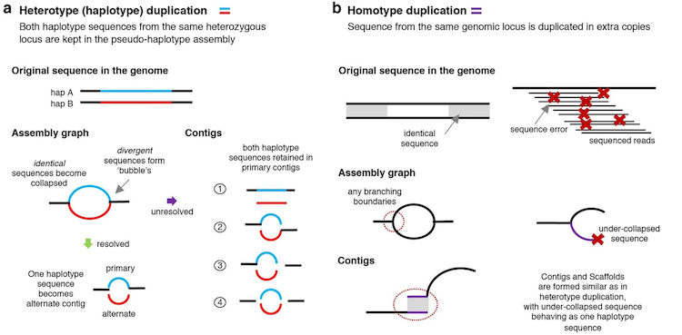 Open image in new tab


:
Warning: Danger: Make sure you choose corect format!

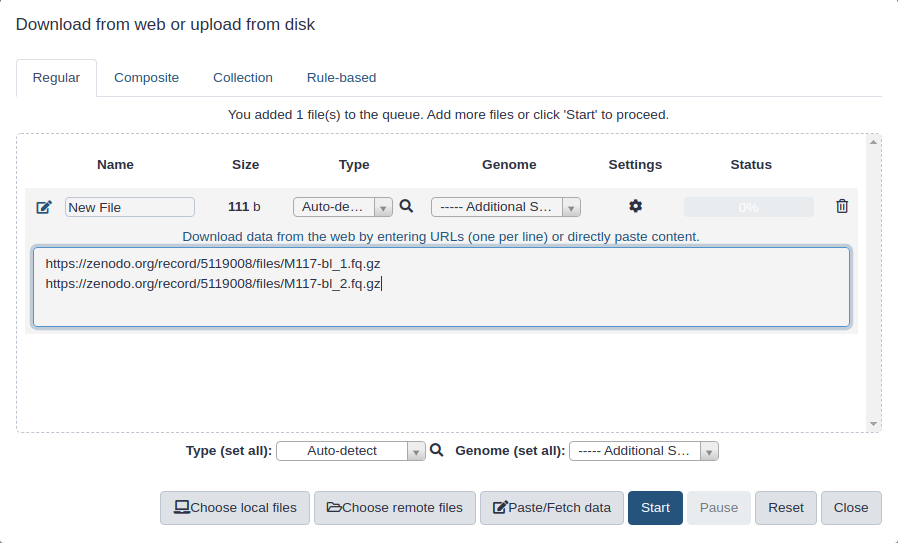


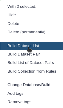


Open image in new tab
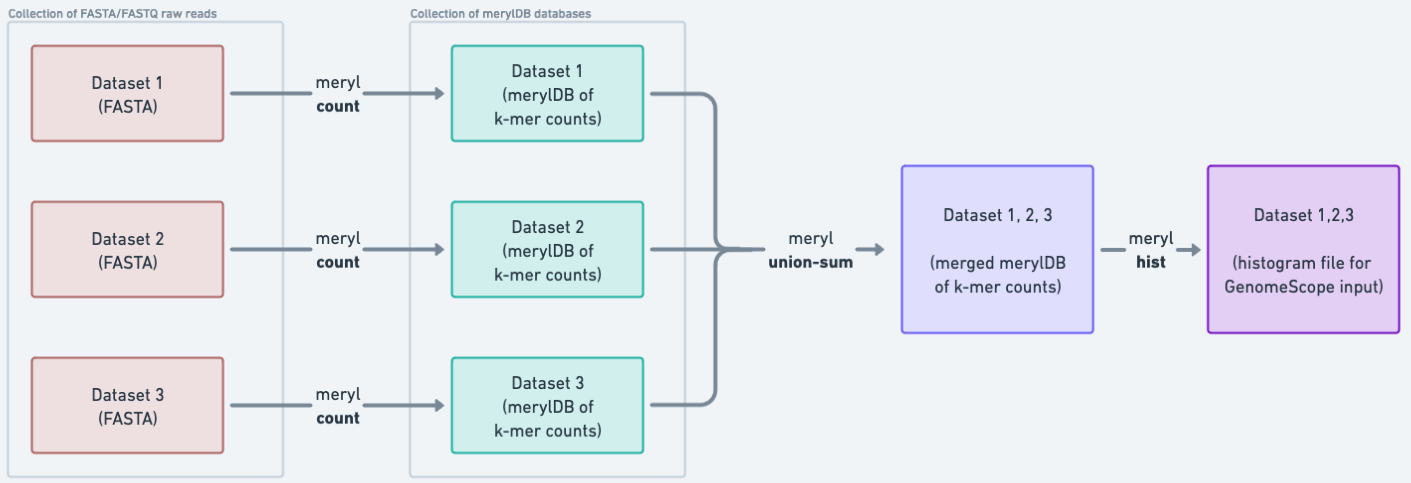 Open image in new tab
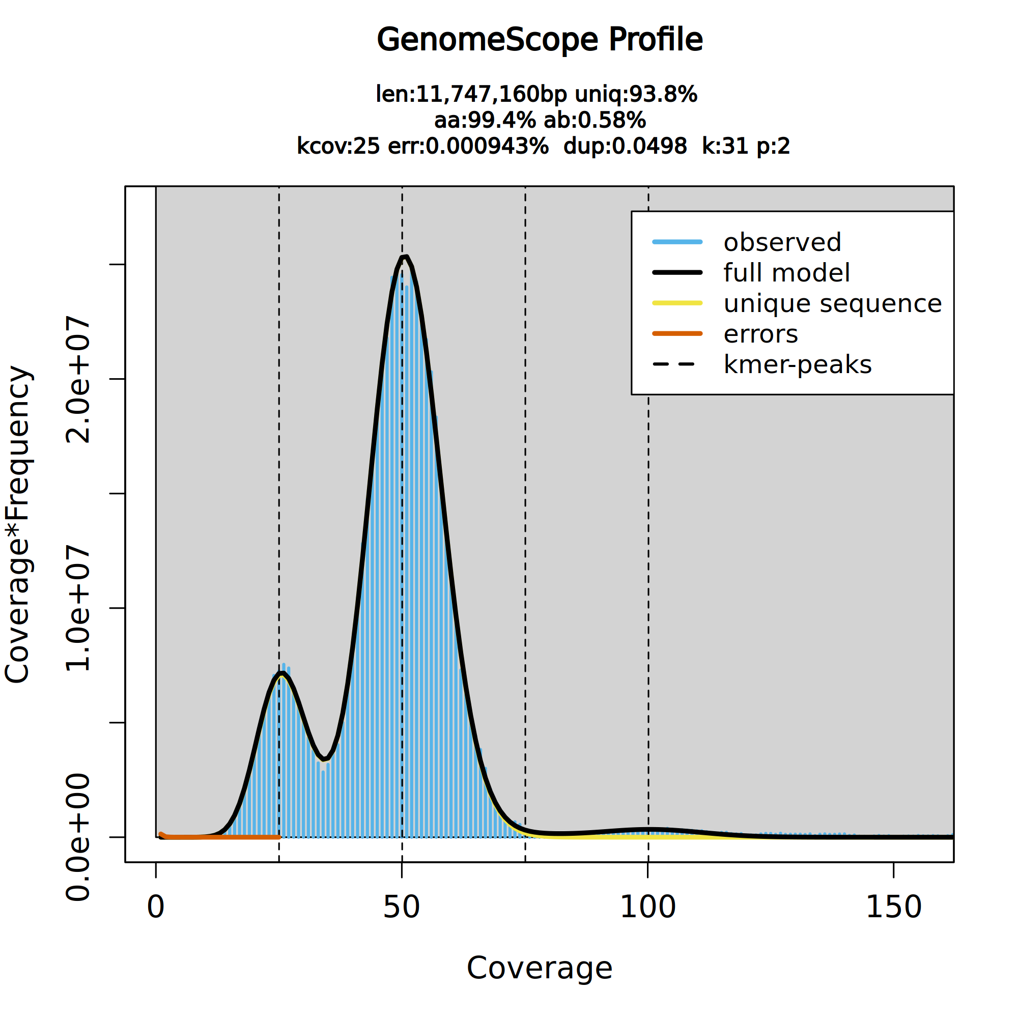 Open image in new tab
Open image in new tab
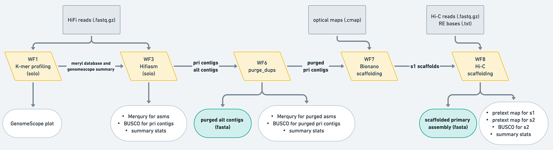 Open image in new tab
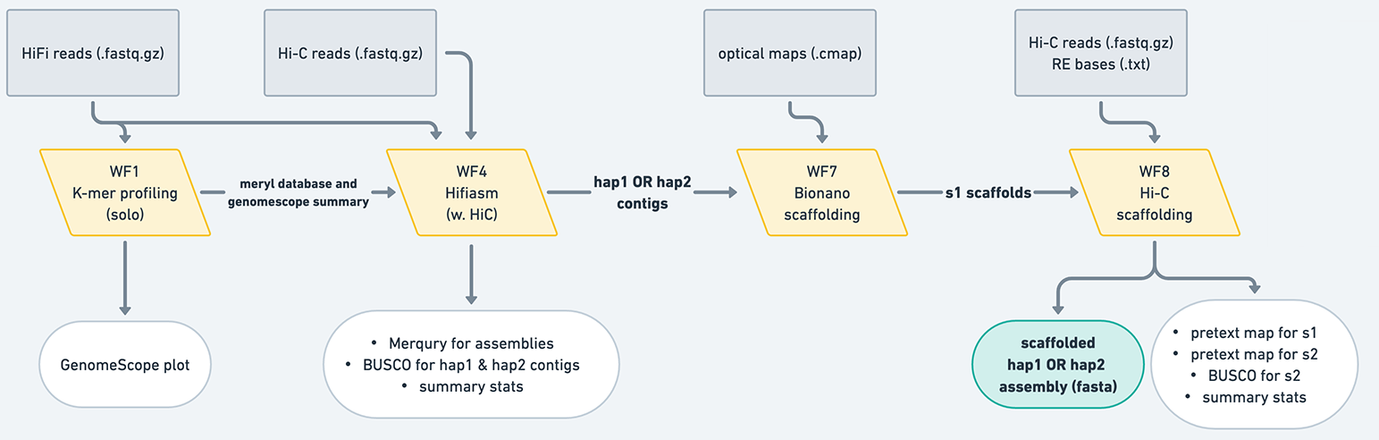 Open image in new tab
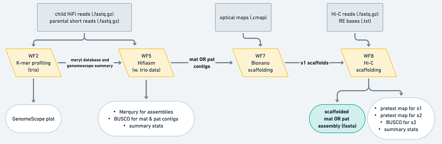 Open image in new tab
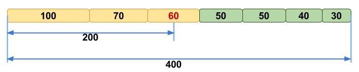 Open image in new tab
Open image in new tab
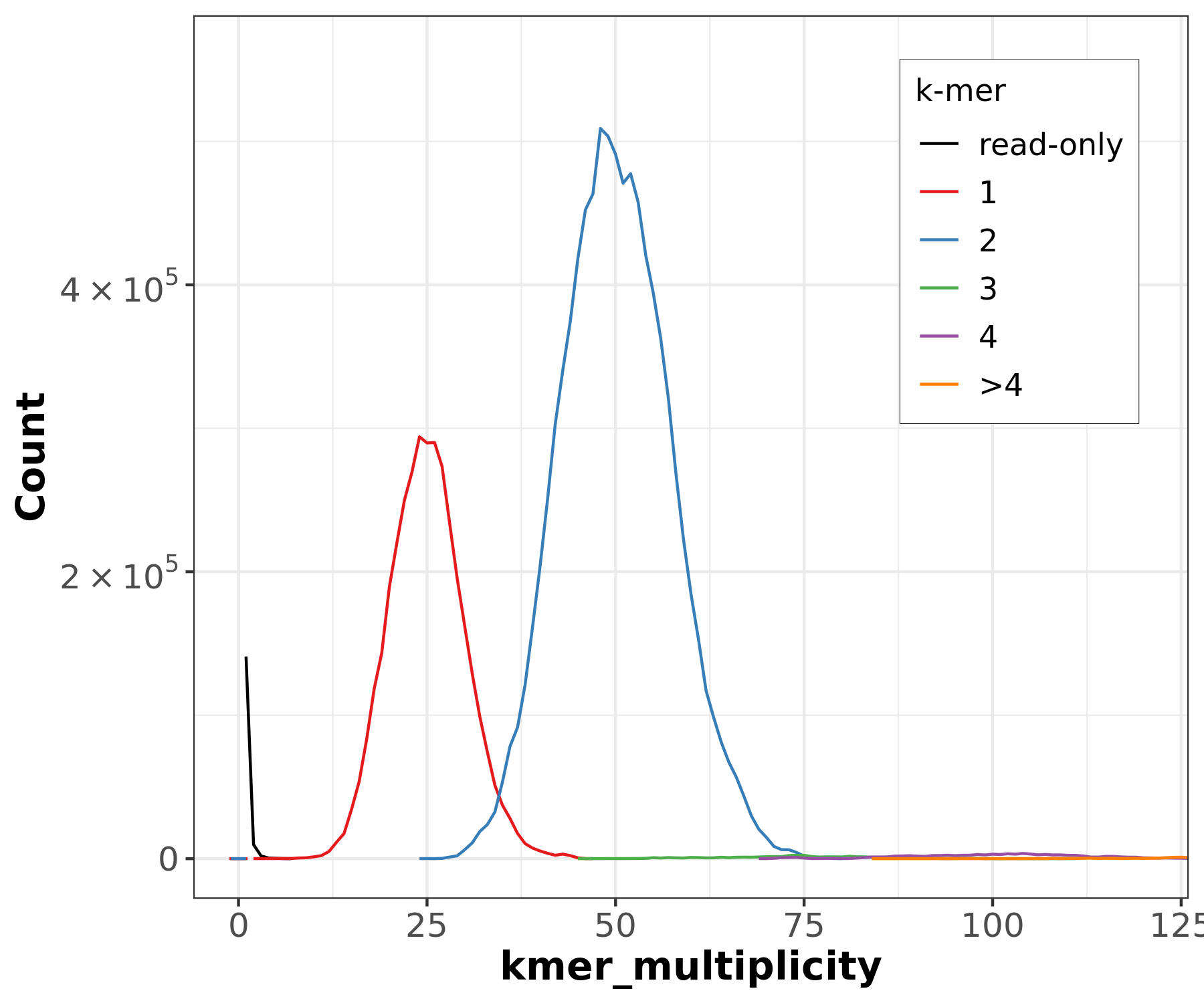 Open image in new tab
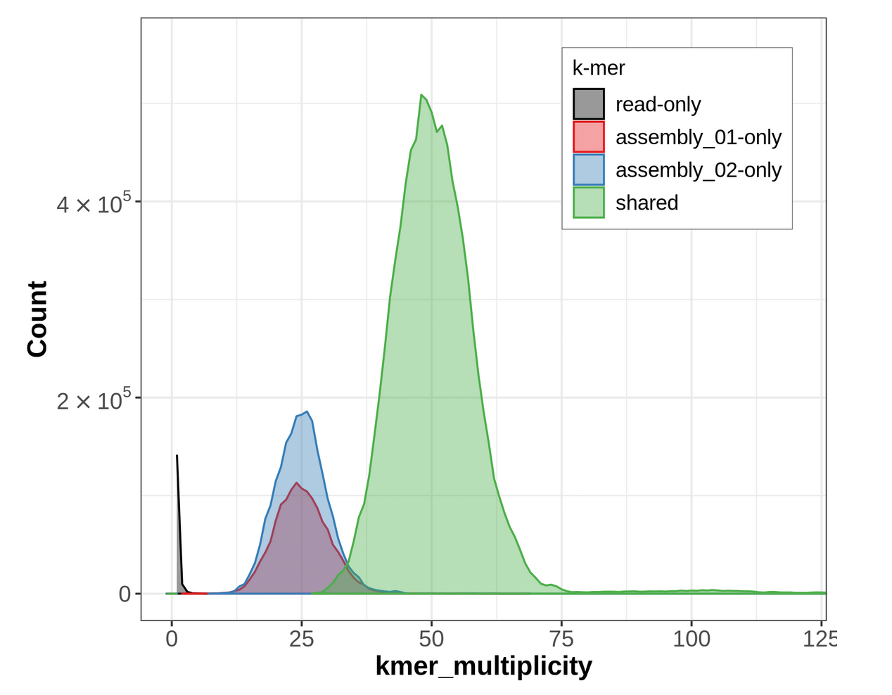 Open image in new tab
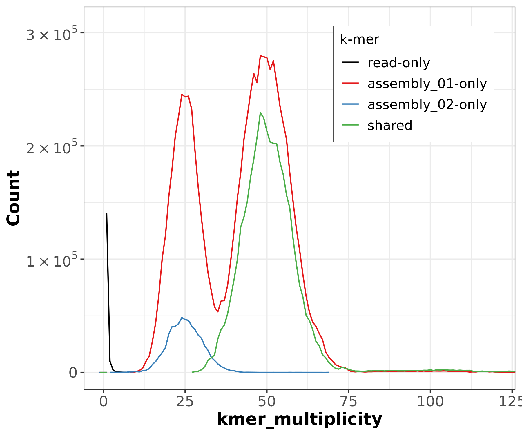 Open image in new tab
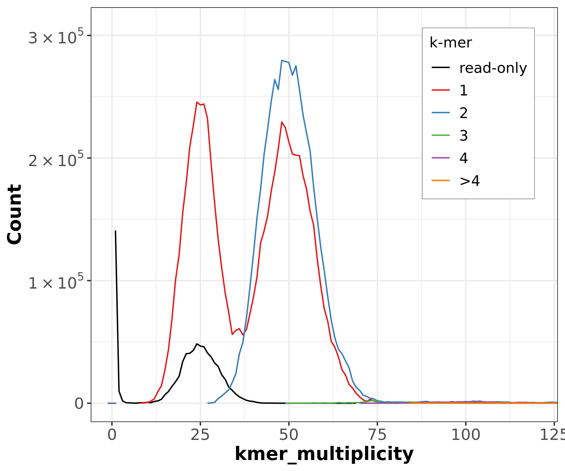 Open image in new tab
Open image in new tab
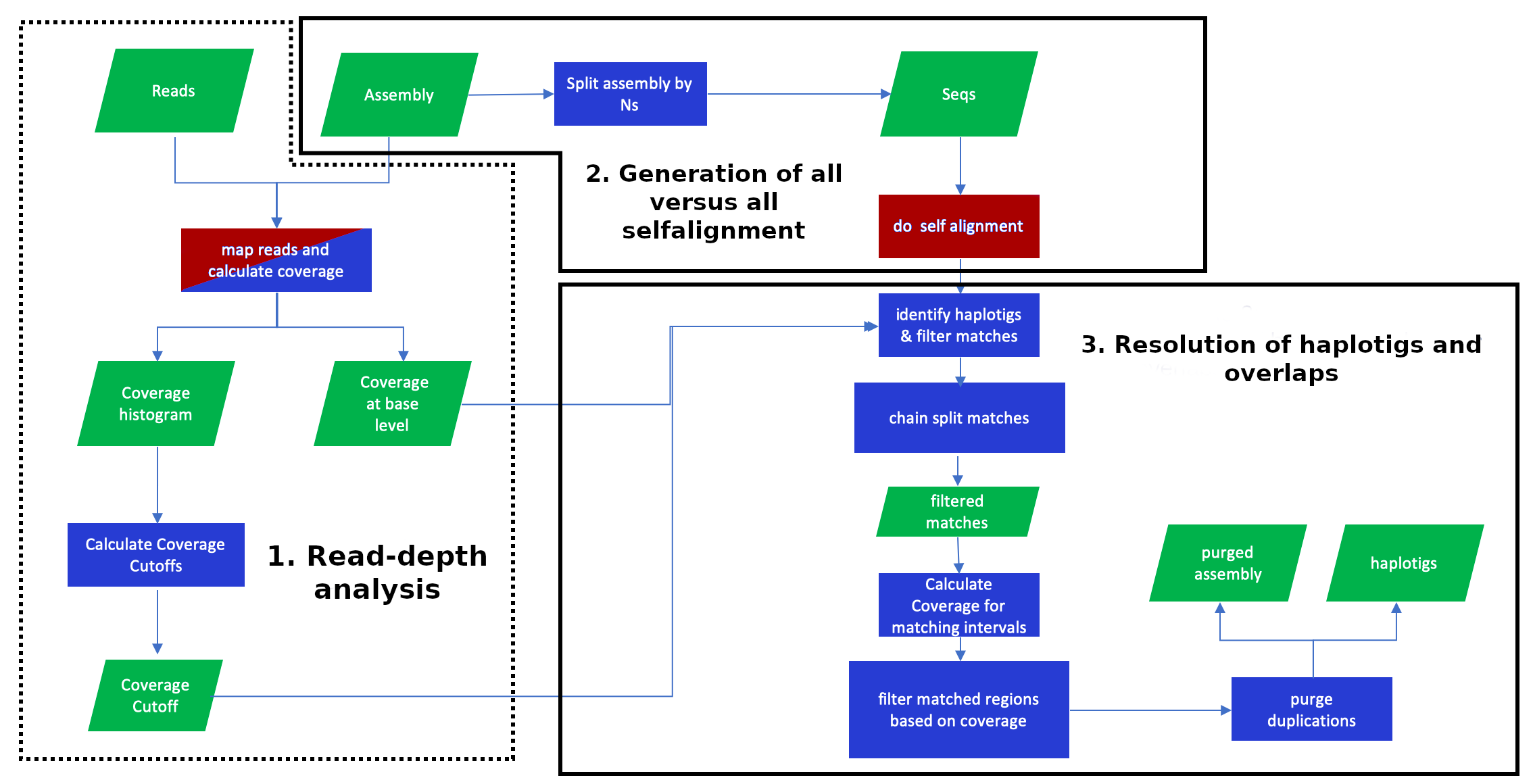 Open image in new tab
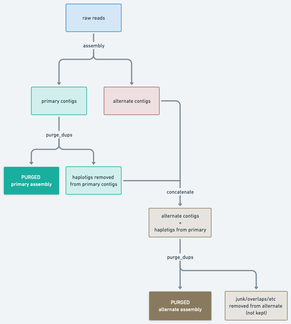 Open image in new tab
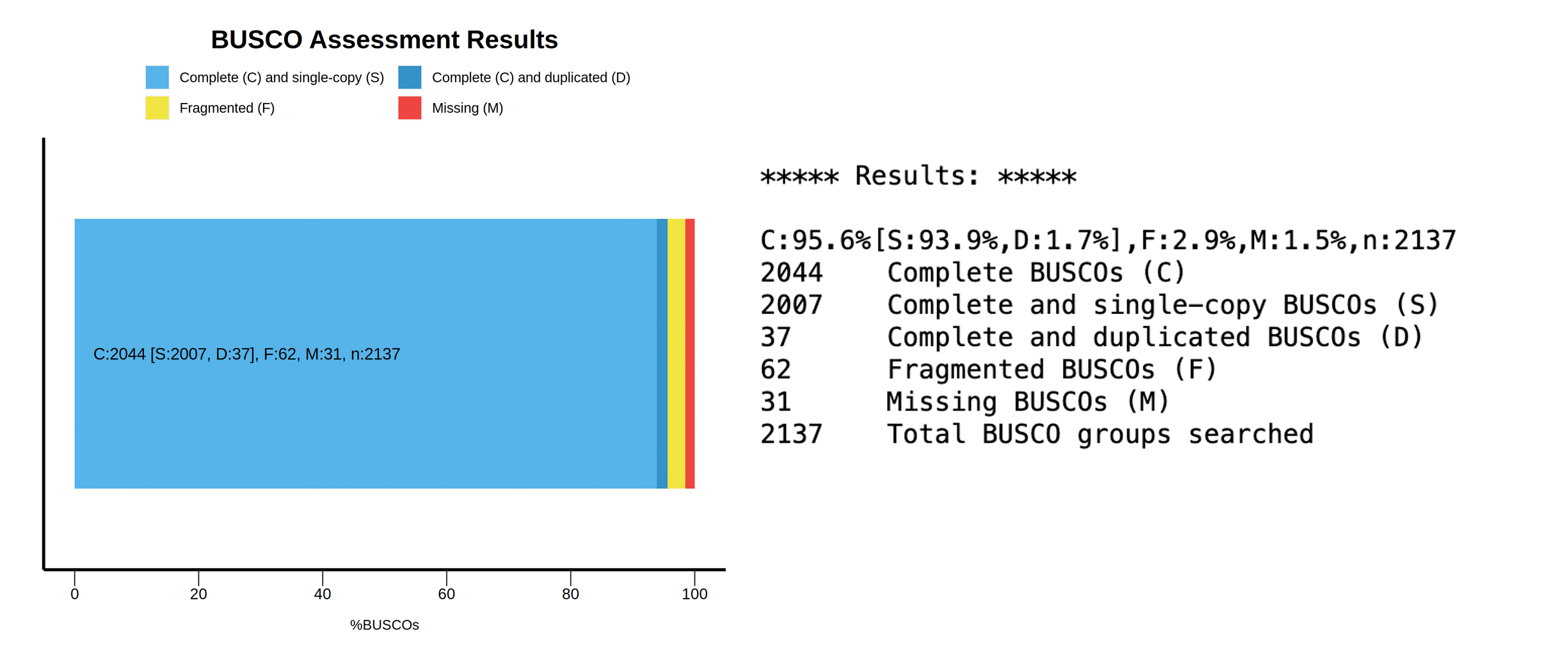 Open image in new tab
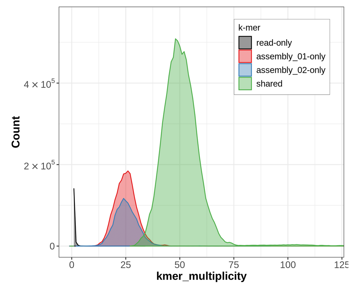 Open image in new tab
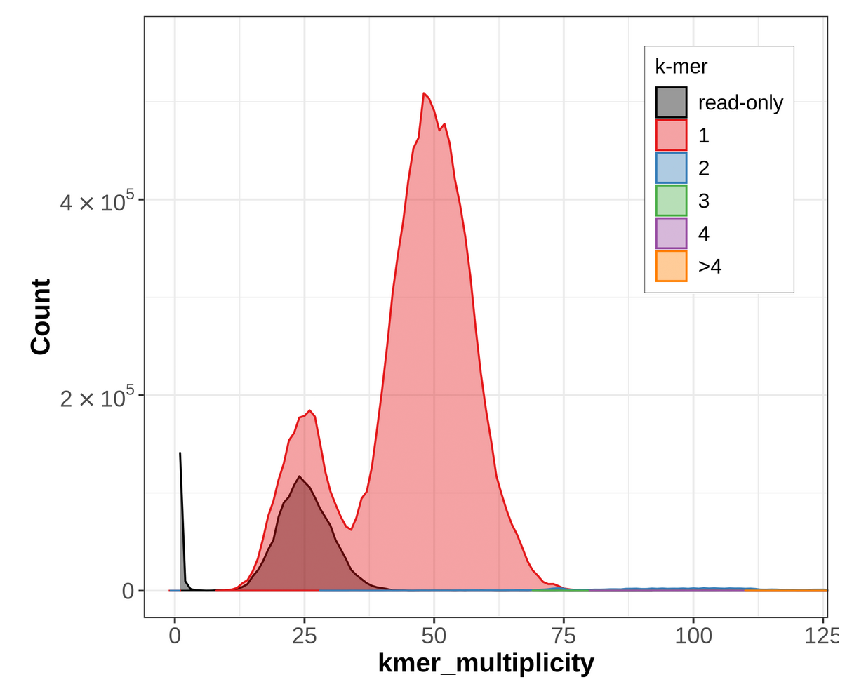 Open image in new tab
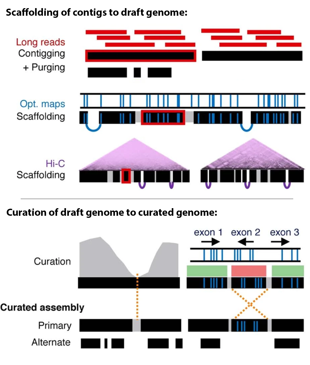 Open image in new tab
Open image in new tab
Open image in new tab
Open image in new tab
Open image in new tab
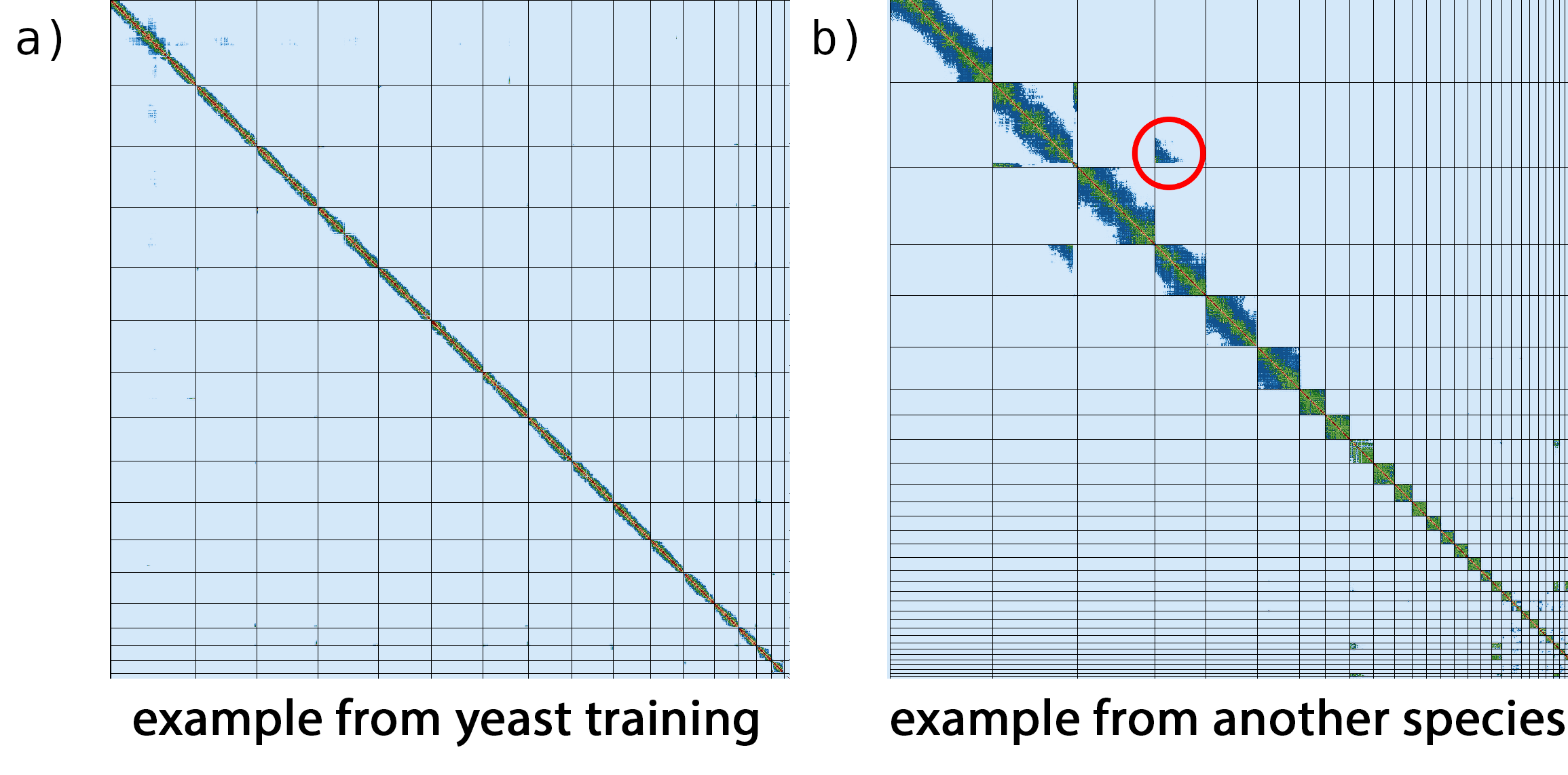 Open image in new tab
Open image in new tab
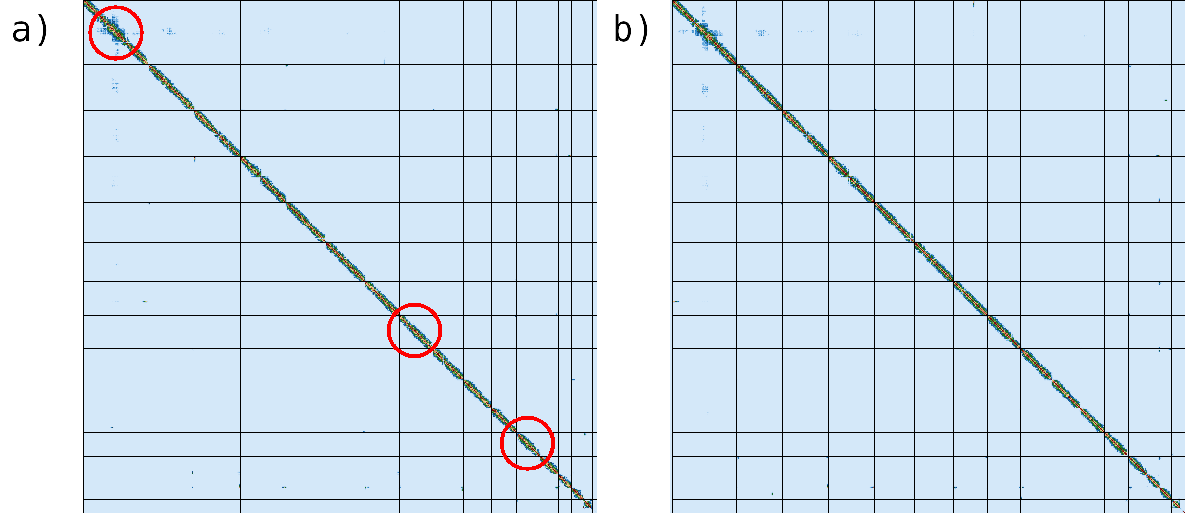 Open image in new tab
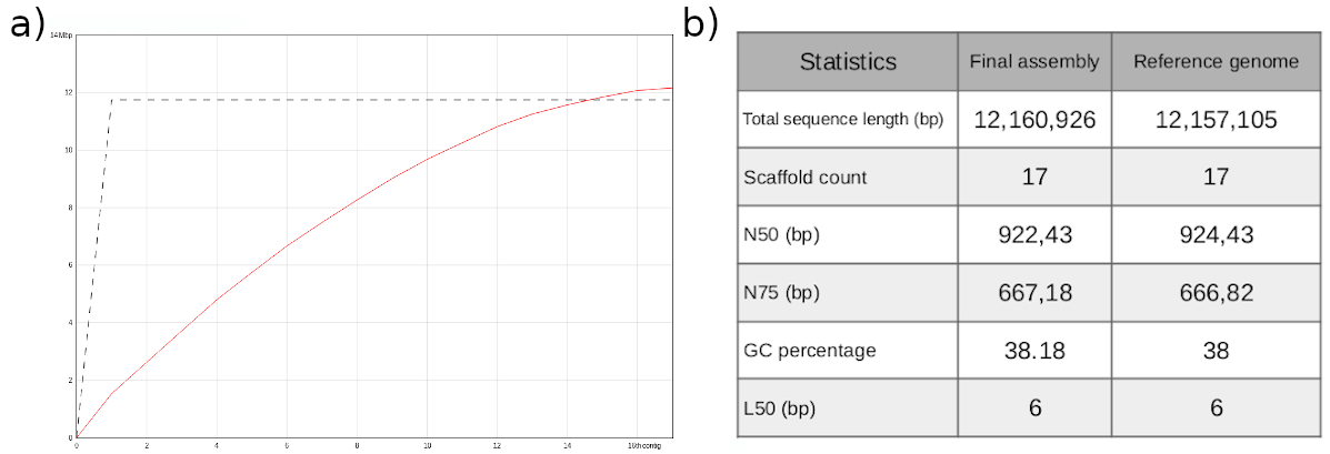 Open image in new tab
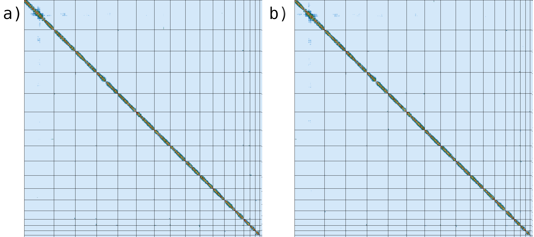 Open image in new tab