Single-cell RNA-seq analysis is a rapidly evolving field at the forefront of transcriptomic research, used in high-throughput developmental studies and rare transcript studies to examine cell heterogeneity within a populations of cells.
The cellular resolution and genome wide scope make it possible to draw new conclusions that are not otherwise possible with bulk RNA-seq. The analysis requires a great deal of knowledge about statistics, wet-lab protocols, and some machine learning due to variability and sparseness of the data. The uncertainty from the low coverage and low cell numbers per sample that once were common setbacks in the field are overcome by 10x Genomics which provides high-throughput solutions which are quickly championing the field.
Era of 10x Genomics
10x genomics has provided not only a cost-effective high-throughput solution to understanding sample heterogeneity at the individual cell level, but has defined the standards of the field that many downstream analysis packages are now scrambling to accommodate.
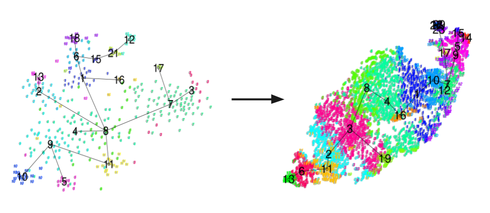
Figure 1: From less than 1K to over 10K with 10x genomics: Analyses of two separate scRNA datasets using the (left) CelSEQ2 protocol, and the (right) 10x Chromium system.
The gain in resolution reduces the granularity and noise issues that plagued the field of scRNA-seq not long ago, where now individual clusters are much easier to decipher due to the added stability added by this gain in information.
The 10X barcoded gel beads consist of a pool barcodes which are used to separately index each cell’s transcriptome. The individual gel barcodes are delivered to each cell via flow-cytometry, where each cell is fed single-file along a liquid tube and tagged with a 10X gel bead. The cells are then isolated from one another within thousands of nanoliter droplets, where each droplet described by a unique 10x barcode that all reads in that droplet are associated with once they undergo reverse-transcription (RT) which reconstructs the mRNA into a cDNA counterpart. The oil is then removed and all (now barcoded) cDNA reads are pooled together to be sequenced.
Though there are approximately 3 million 10x gel barcodes used, the amount actually qualitatively profiled in a sample is ~10,000 due to majority of droplets (>90%) being empty in order to ensure that the remainder contains only one cell.
There are actually two sets of barcodes for the different chemistries provided; one which has 737,000 barcodes, and one with ~3,7 million barcodes.
Both are provided in the Zenodo link, but we will only work with the 3 million barcodes because this is what is provided with the chemistry version.
If you are getting a low number of cells detected for your reads later on, it could be because the barcodes provided are wrong.
The first part of this tutorial is essentially a one-click “fire and forget” solution to demultiplexing and quantifying scRNA-seq data, where much of the complexity required in this extremely crucial stage is simplified into a single step.
However, those who are more interested in learning the intricacies of how FASTQ files are transformed into a count matrix, please see the Pre-processing of Single-Cell RNA Data tutorial.
10x Genomics has its own processing pipeline, Cell Ranger to process the scRNA-seq outputs it produces, but this process requires much configuration to run and is significantly slower than other mappers.
Since STARsolo is a drop-in solution to the Cell Ranger pipeline, the first part of the tutorial is a one-click solution where users are encouraged to launch their RNA STARsolo jobs and spend the time familiarising themselves with the pre-processing training materials mentioned above.
Figure 4: Benchmark of different mapping software.
The image is from Melsted et al. 2019. Notice the order of magnitude speed up that STARsolo and a few others display, for a variety of different datasets in comparison to Cell Ranger.
The second part of this tutorial also has a one-click solution to producing a matrix identical to that given by the Cell Ranger pipeline, but the more interesting aspects of the pipeline are explored in the Introspective Method part of the tutorial.
Producing a Count Matrix from FASTQ
Here we will use the 1k PBMCs from a Healthy Donor (v3 chemistry) from 10x genomics, consisting of 1000 Peripheral blood mononuclear cells (PBMCs) extracted from a healthy donor, where PBMCs are primary cells with relatively small amounts of RNA (~1pg RNA/cell).
The source material consists of 6 FASTQ files split into two sequencing lanes L001 and L002, each with three reads of R1 (barcodes), R2 (cDNA sequences), I1 (illumina lane info):
pbmc_1k_v3_S1_L001_R1_001.fastq.gz
pbmc_1k_v3_S1_L001_R2_001.fastq.gz
pbmc_1k_v3_S1_L001_I1_001.fastq.gz
pbmc_1k_v3_S1_L002_R1_001.fastq.gz
pbmc_1k_v3_S1_L002_R2_001.fastq.gz
pbmc_1k_v3_S1_L002_I1_001.fastq.gz
The Cell Ranger pipeline requires all three files to perform the demultiplexing and quantification, but RNA STARsolo does not require the I1 lane file to perform the analysis. These source files are provided in the Zenodo data repository, but they require approximately 2 hours to process. For this tutorial, we will use datasets sub-sampled from the source files to contain approximately 300 cells instead of 1000. Details of this sub-sampling process can be viewed at the Zenodo link.
Data upload and organization
For the mapping, we require the sub-sampled source files, as well as a “whitelist” of (~3,7 million) known cell barcodes, freely extracted from the Cell Ranger pipeline. This whitelist file may be found within the Galaxy Data Library, but it is included here in the Zenodo record for convenience and also because the sequencing facility may not always provide this file.
The barcodes in the R1 FASTQ data are checked against these known cell barcodes in order assign a specific read to a specific known cell. The barcodes are designed in such a manner that there is virtually no chance that they will align to a place in the reference genome. In this tutorial we will be using hg19 (GRCh37) version of the human genome, and will therefore also need to use a hg19 GTF file to annotate our reads.
Hands On: Data upload and organization
Create a new history and rename it (e.g. scRNA-seq 10X dataset tutorial)
To create a new history simply click the new-history icon at the top of the history panel:
Import the sub-sampled FASTQ data from Zenodo or from the data library (ask your instructor)
As an alternative to uploading the data from a URL or your computer, the files may also have been made available from a shared data library:
Go into Libraries (left panel)
Navigate to the correct folder as indicated by your instructor.
On most Galaxies tutorial data will be provided in a folder named GTN - Material –> Topic Name -> Tutorial Name.
Select the desired files
Click on Add to Historygalaxy-dropdown near the top and select as Datasets from the dropdown menu
In the pop-up window, choose
“Select history”: the history you want to import the data to (or create a new one)
There are two main reagent kits used during the library preparation, and the choice of one will influence the size of the sequences we work with. Below we can see the layout of the primers used in both chemistries. We can ignore most of these as they are not relevant, namely: the P5 and P7 illumina primers are used in the illumina bridge amplification process; the Sample Index is an 8bp primer which is related to the Chromium system that balances nucleotide bias and ensures that there is no sample overlap during the multiplexed sequencing; and the Poly(dT) VN primer used to capture RNA sequences with poly-A tails (i.e. mRNA).
Figure 5: 10x Chromiumv2 and Chromiumv3 Chemistries
The primers of interest to us are the Cell Barcode (CB) and the Unique Molecular Identifiers (UMI) used in the Read 1 sequencing primer, as they describe to us how to demultiplex and deduplicate our reads. It is highly advised that the Plates, Batches, and Barcodes slides are revisited to refresh your mind on these concepts.
Chemistry
Read 2
Read 1 (CB + UMI)
Insert (Read 2 + Read 1)
v2
98
26 (16 + 10)
124
v3
91
28 (16 + 12)
119
The table above gives a summary of the primers used in the image and the number of basepairs occupied by each.
Unstranded protocols do not distinguish between whether a fragment was sequenced from the forward or the reverse strand, which can lead to some ambiguity if the fragment overlaps two transcripts. In the image below, it is not clear whether the fragment is derived from GeneF or GeneR due to this overlap.
Figure 6: Mapping fragments to overlapping transcripts is ambiguous with unstranded protocols.
Stranded protocols overcome this by fitting different 5’ and 3’ primers and adaptors, meaning that the orientation of the fragment is fixed during sequencing. For the Chromium v2 and v3 chemistries, the barcode information is purely within the R1 forward strand.
Question
What has stayed constant between the chemistry versions?
What advantage does this constant factor give?
What do UMIs do?
What advantage does the 2 extra bp in the v3 UMIs have over v2 UMIs?
What will be the strandedness of the generated library
The Cell Barcode (CB) has remained at 16bp for both chemistries.
This has the advantage that the same set of barcodes can be used in both chemistries, which is important because barcodes are very hard to design.
They need to be designed in such a way to minimise accidentally aligning to the reference they were prepared to be used for.
Longer barcodes tend to be more unique, so this is a problem that is being solved as the barcodes increase in size, allowing for barcodes that can be used on more than one reference to be more common, as seen above.
UMIs (or Unique Molecular identifiers) do not delineate cells as Cell Barcodes do, but instead serve as random ‘salt’ that tag molecules randomly and are used to mitigate amplification bias by deduplicating any two reads that map to the same position with the same UMI, where the chance of this happening will be astronomically small unless one read is a direct amplicon of the other.
\(4^{10} = 1,048,576\) unique molecules tagged, vs. \(4^{12} = 16,777,216\) unique molecules tagged. The reality is much much smaller due to edit distances being used that would reduce both these numbers substantially (as seen in the Plates, Batches, and Barcodes slides), but the scale factor of 16 times more molecules (\(4^{12-10} = 16\)) can be uniquely tagged is true.
Forward.
The differences in the chemistries is a slight change in the library size, where the v2 aims to capture on average 50,000 reads per cell, whereas the v3 aims to capture at minimum 20,000 reads per cell. This greatly reduces the lower-tail of the library size compared to the previous version.
Determining what Chemistry our Data Contains
To perform the demultiplexing, we need to tell RNA STARsolo where to look in the R1 FASTQ to find the cell barcodes. We can do this by simply counting the number of basepairs in any read of the R1 files.
Question
Peek at one of the R1 FASTQ files using the galaxy-eye symbol below the dataset name.
How many basepairs are there in any given read?
Which library preparation chemistry version was this read generated from?
There are 28 basepairs.
The v2 has 26 basepairs, but the v3 has 28 basepairs. Therefore the reads we have here use the Chromium v3 chemistry.
Performing the Demultiplexing and Quantification
We will now proceed to demultiplex, map, and quantify both sets of reads using the correct chemistry discovered in the previous sub-section.
Comment
RNA STARsolo ( Galaxy version 2.7.10b+galaxy3) consumes a large amount of memory. During the Smörgåsbord training please use Human (Homo Sapiens): hg19 chrX as the reference genome if you follow this tutorial on usegalaxy.org. This performs the mapping only against chromosome X. The full output dataset is available at zenodo and will be the starting point for the next tutorial.
Hands On
RNA STARsolo ( Galaxy version 2.7.11a+galaxy1) with the following parameters:
“Custom or built-in reference genome”: Use a built-in index
“Reference genome with or without an annotation”: use genome reference without builtin gene-model
“Select reference genome”: Human (Homo Sapiens): hg19 Full or Human (Homo Sapiens) (b37): hg19
“Gene model (gff3,gtf) file for splice junctions”: Homo_sapiens.GRCh37.75.gtf
“Length of genomic sequence around annotated junctions”: 100
“Type of single-cell RNA-seq”: Drop-seq or 10X Chromium
“Input Type”: Separate barcode and cDNA reads
param-file“RNA-Seq FASTQ/FASTA file, Barcode reads”: Multi-select L001_R1_001 and L002_R1_001 using the Ctrl key.
param-file“RNA-Seq FASTQ/FASTA file, cDNA reads”: Multi-select L001_R2_001 and L002_R2_001 using the Ctrl key.
“Type of UMI filtering”: Remove UMIs with N and homopolymers (similar to CellRanger 2.2.0)
“Matching the Cell Barcodes to the WhiteList”: Multiple matches (CellRanger 2, 1MM_multi)
Under “Advanced Settings”:
“Strandedness of Library”: Read strand same as the original RNA molecule
“Collect UMI counts for these genomic features”: Gene: Count reads matching the Gene Transcript
“Cell filter type and parameters”: Do not filter
“Field 3 in the Genes output”: Gene Expression
Comment
The in-built Cell filtering is a relatively new feature that emulates the CellRanger pipeline. Here, we set the filtering options to not filter because we will use our own methods to better understand how this works. For your own future datasets, you may wish to enable the filtering parameter.
Inspecting the Output Files
At this stage RNA STARsolo has output 6 files; a program log, a mapping quality file, a BAM file of alignments, and 3 count matrix files:
Log
Feature Statistic Summaries
Alignments
Matrix Gene Counts
Barcodes
Genes
The log and the summaries files give program logistics and metrics about the quality of the mapping. The BAM file contains the reads mapped to the reference genome. The matrix gene counts is the count matrix in matrixmarket format, accompanied by the list of genes and cell barcodes in separate files. These can be converted into tabular or AnnData formats using the toolImport Anndata and loom tool.
Mapping Quality
Let us investigate the output log. This type of quality control is essential in any RNA-based analysis and it is strongly recommended that you familiarise yourself with the Quality Control tutorial.
Hands On
MultiQC ( Galaxy version 1.27+galaxy0) with the following parameters:
In “Results”:
In “1:Results”:
“Which tool was used generate logs?”: STAR
In “STAR output”:
In “1:STAR output”:
“Type of STAR output?”: Log
param-file“STAR log output”: RNA STARsolo: log
Question
What percentage of reads are uniquely mapped?
87.5%
This is good, and is expected of 10x datasets.
Quantification Quality
The above tool provides a nice visualisation of the output log, and is a fantastic way to combine multiple quality sources into one concise report.
However, sometimes it is often more informative to look directly at the source quality control file. For example, let us investigate the STARsolo Feature summaries file.
We can look at this directly by clicking on the galaxy-eye symbol of the Feature Statistic Summaries file.
The explanation of these parameters can be seen in the RNA STAR Manual under the STARsolo section, with most of the information given in the details box below.
Parameter
Explanation
noNinCB
number of reads with more than 2 Ns in cell barcode (CB)
noUMIhomopolymer
number of reads with homopolymer in CB
noTooManyWLmatches
(not used at the moment)
noNoWLmatch
number of reads with CBs that do not match whitelist even with one mismatch
All of the above reads are discarded from Solo output.
The remaining reads are checked for any overlap with the features/genes:
Parameter
Explanation
noUnmapped
number of reads unmapped to the genome
noNoFeature
number of reads that map to the genome but do not belong to a feature
MultiFeature
number of reads that belong to more than one feature
subMultiFeatureMultiGenomic
number of reads that belong to more than one feature and are also multimapping to the genome (this is a subset of the nAmbigFeature)
noTooManyWLmatches
number of reads with ambiguous CB (i.e. CB matches whitelist with one mismatch but with posterior probability 0.95)
noMMtoWLwithoutExact
number of reads with CB that matches a whitelist barcode with 1 mismatch, but this whitelist barcode does not get any other reads with exact matches of CB
These metrics can be grouped into more broad categories:
noNinCB + noUMIhomopolymer + noNoWLmatch + noTooManyWLmatches + noMMtoWLwithoutExact = number of reads with CBs that do not match whitelist.
noUnmapped + MultiFeature = number of reads without defined feature (gene).
yessubWLmatch_UniqueFeature = number of reads that are output as solo counts.
The three categories above summed together should be equal to the total number of reads (which is also given in the MultiQC output).
The main information to gather at this stage is that the yesCellBarcodes tell us how many cells were detected in our sample, where we see that there are 5200 cells. Another metric to take into account is that the number of matches (yessubWLmatch_UniqueFeature) has the largest value, and that the number of reads that map to the genome but not to a feature/gene given in the GTF (noNoFeature) is not too large. The number of no features is also quite high when mapping the original (non-subsampled) 10x input datasets, so this appears to be the default expected behaviour.
Producing a Quality Count Matrix
The matrix files produced by RNA STARsolo are in the bundled format, meaning that the information to create a tabular matrix of Genes vs Cells are separated into different files. These files are already 10x analysis datasets, compatible with any downstream single-cell RNA analysis pipeline, however the number of cells represented here are greatly over-represented, as they have not yet been filtered for high quality cells, and therefore the matrix represents any cells that were unambiguously detected in the sample.
If we were to construct a cell matrix using the data we have, we would have a large matrix of 60,000 Genes against 3 million Cells, of which most values would be zero, i.e. an extremely sparse matrix.
To get a high quality count matrix we must apply the DropletUtils tool, which will produce a filtered dataset that is more representative of the Cell Ranger pipeline.
Cell Ranger Method
Hands On: Default Method
DropletUtils ( Galaxy version 1.10.0+galaxy2) with the following parameters:
“Format for the input matrix”: Bundled (barcodes.tsv, genes.tsv, matrix.mtx)
param-file“Count Data”: Matrix Gene Counts (output of RNA STARsolotool)
param-file“Genes List”: Genes (output of RNA STARsolotool)
param-file“Barcodes List”: Barcodes (output of RNA STARsolotool)
“Operation”: Filter for Barcodes
“Method”: DefaultDrops
“Expected Number of Cells”: 3000
“Upper Quantile”: 0.99
“Lower Proportion”: 0.1
“Format for output matrices”: Bundled (barcodes.tsv, genes.tsv, matrix.mtx)
Comment: Default Parameter
The “Expected Number of Cells” parameter is the number of cells you expect to see in your sample, but does not correspond to how many cells you expect to see in a sub-sampled dataset like this one. The default is 3000 for Cell Ranger, which will yield ~300 cells here, but users are encouraged to experiment with this value when dealing with their own data, to recover the desired number of cells.
Question
How many cells were detected?
Does this agree with the STARsolo Feature Statistics output?
By clicking on the title of the output dataset in the history we can expand the box to see the output says that there are 272 cells in the output table.
If we expand the galaxy-eyeRNA STARsolo Feature Statistic Summaries Dataset and look at the yesCellBarcodes value, we see that RNA STARsolo detected 5200 cells. What this means is that 5200 barcodes were detected in total, but only 272 of them were above an acceptable threshold of quality, based on the default upper quantile and lower proportion parameters given in the tool. Later on, we will actually later visualise these thresholds ourselves by “ranking” the barcodes, to see the dividing line between high and low quality barcodes.
This will produce a count matrix in a human readable tabular format which can be used in downstream analysis tools, such as those used in the Downstream Single-cell RNA analysis with RaceID tutorial.
The tabular outputs here are selected mostly for transparency, since they are easy to inspect. However, the datasets produced with 10x data are very large and very sparse, meaning there is much data redundancy due to the repetition of zeroes everywhere in the data.
Many analysis packages have attempted to solve this problem by inventing their own standard, which has led to the proliferation of many different “standards” in the scRNA-seq package ecosystem, most of which require an R programming environment to inspect.
As expected, the format that usually wins is the one which is most common in the field. In this case, the format also happens to be a very good format that stores data in a concise, compressed, and extremely readable manner:
<img src=”/training-material/topics/single-cell/images/scrna-pre-processing/tenx_anndata.svg “AnnData is an HDF5-based format, which stores gene and cell information in their own matrices, complementary to the main data matrix.” “ alt=”anddata. “ width=”194” height=158 loading=”lazy”>
The AnnData format (hda5) is an extension of the HDF5 format, which supports multidimensional datasets to be stored in a consistent and space-optimised way. This is the default output of Cell Ranger and so is also the default output of RNA STARsolo. The format is also now a widely accepted format in many downstream analysis suites.
Introspective Method
The DefaultDrops method given in the previous sub-section is a good one-click solution to emulating the Cell Ranger process of producing a high quality count matrix.
However, the DropletUtils tool does provide other options for determining which cells are of “good” quality and which are not.
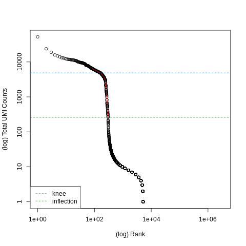
A useful diagnostic for droplet-based data is the barcode rank plot, which shows the (log-)total UMI count for each barcode on the y-axis and the (log-)rank on the x-axis. This is effectively a transposed empirical cumulative density plot with log-transformed axes. It is useful as it allows users to examine the distribution of total counts across barcodes, focusing on those with the largest counts.
Hands On: Rank Barcodes
DropletUtils ( Galaxy version 1.10.0+galaxy2) with the following parameters:
“Format for the input matrix”: Bundled (barcodes.tsv, genes.tsv, matrix.mtx)
param-file“Count Data”: Matrix Gene Counts (output of RNA STARsolotool)
param-file“Genes List”: Genes (output of RNA STARsolotool)
param-file“Barcodes List”: Barcodes (output of RNA STARsolotool)
Figure 7: Barcode Ranks: The separating thresholds of high and low quality cells
The knee and inflection points on the curve mark the transition between two components of the total count distribution. This is assumed to represent the difference between cells with high RNA content and empty droplets with little RNA, and gives us a rough idea of how many cells to expect in our sample.
Question question Questions
How many presumably real cells can we expect to see in our sample based on the above plot?
What is the number of cells that we can expect to see with a cut-off detected at inflection line?
We see the blue knee line cross the threshold of barcodes at just below than the 10000 Rank on the horizontal log scale, which is shown in the expanded view of our data as "knee = 4861". This line intersects with the ranked cells near 100 on x-axis. We can expect 100-200 cells with high RNA content.
This threshold is given by the inflection line, which is given at "inflection = 260". The vertical drop in the ranked cells at the inflection line is between 100 and 10000 on the x-axis. The axis is log scaled it is close to 100. Hence, we can expect between 200 and 400 cells.
On large 10x datasets we can use these thresholds as metrics to utilise in our own custom filtering, which is once again provided by the DropletUtils tool. In this case, we will use a bit less stringent threshold of 200 (instead of 260 at inflection) and use a FDR threshold of 0.01 so that our detected cells contain only 1% of false positives.
Hands On: Custom Filtering
DropletUtils ( Galaxy version 1.10.0+galaxy2) with the following parameters:
“Format for the input matrix”: Bundled (barcodes.tsv, genes.tsv, matrix.mtx)
param-file“Count Data”: Matrix Gene Counts (output of RNA STARsolotool)
param-file“Genes List”: Genes (output of RNA STARsolotool)
param-file“Barcodes List”: Barcodes (output of RNA STARsolotool)
“Operation”: Filter for Barcodes
“Method”: EmptyDrops
“Lower-bound Threshold”: 200
“FDR Threshold”: 0.01
“Format for output matrices”: Bundled (barcodes.tsv, genes.tsv, matrix.mtx)
Here we recover 279 high quality cells instead of the 272 detected via the default method previously. On large datasets, this difference can help clean downstream clustering. For example, soft or less well-defined clusters are derived from too much noise in the data due to too many low quality cells being in the data during the clustering. Filtering these out during the pre-processing would produce much better separation, albeit at the cost of having less cells to cluster. This filter-cluster trade-off is discussed in more detail in the downstream analysis training materials.
Conclusion
In this workflow we have learned to quickly perform mapping and quantification of scRNA-seq FASTQ data in a single step via RNA STARsolo, and have reproduced a Cell Ranger workflow using the DropletUtils suite, where we further explored the use of barcode rankings to determine better filtering thresholds to generate a high quality count matrix.
A full pipeline which produces both an AnnData and tabular file for inspection is provided in this workflow
Note that, since version 2.7.7a of the tool, the entire Cell Ranger pipeline including the filtering can be performed natively within RNA STARsolo. As this is still a relatively new feature, we do not use it here in this tutorial, but eager users are encouraged to try it out.
This tutorial is part of the https://singlecell.usegalaxy.eu portal (Tekman et al. 2020).
You've Finished the Tutorial
Please also consider filling out the Feedback Form as well!
Key points
Barcode FASTQ Reads are used to parse cDNA sequencing Reads.
A raw matrix is too large to process alone, and need to be filtered into a high quality one for downstream analysis
Frequently Asked Questions
Have questions about this tutorial? Have a look at the available FAQ pages and support channels
Further information, including links to documentation and original publications, regarding the tools, analysis techniques and the interpretation of results described in this tutorial can be found here.
References
Melsted, P., A. S. Booeshaghi, F. Gao, E. Beltrame, L. Lu et al., 2019 Modular and efficient pre-processing of single-cell RNA-seq. 10.1101/673285
Did you use this material as an instructor? Feel free to give us feedback on how it went.
Did you use this material as a learner or student? Click the form below to leave feedback.
Hiltemann, Saskia, Rasche, Helena et al., 2023 Galaxy Training: A Powerful Framework for Teaching! PLOS Computational Biology 10.1371/journal.pcbi.1010752
Batut et al., 2018 Community-Driven Data Analysis Training for Biology Cell Systems 10.1016/j.cels.2018.05.012
@misc{single-cell-scrna-preprocessing-tenx,
author = "Mehmet Tekman and Hans-Rudolf Hotz and Daniel Blankenberg and Pavankumar Videm",
	title = "Pre-processing of 10X Single-Cell RNA Datasets (Galaxy Training Materials)",
	year = "",
	month = "",
	day = "",
	url = "\url{https://training.galaxyproject.org/training-material/topics/single-cell/tutorials/scrna-preprocessing-tenx/tutorial.html}",
	note = "[Online; accessed TODAY]"
}
@article{Hiltemann_2023,
	doi = {10.1371/journal.pcbi.1010752},
	url = {https://doi.org/10.1371%2Fjournal.pcbi.1010752},
	year = 2023,
	month = {jan},
	publisher = {Public Library of Science ({PLoS})},
	volume = {19},
	number = {1},
	pages = {e1010752},
	author = {Saskia Hiltemann and Helena Rasche and Simon Gladman and Hans-Rudolf Hotz and Delphine Larivi{\`{e}}re and Daniel Blankenberg and Pratik D. Jagtap and Thomas Wollmann and Anthony Bretaudeau and Nadia Gou{\'{e}} and Timothy J. Griffin and Coline Royaux and Yvan Le Bras and Subina Mehta and Anna Syme and Frederik Coppens and Bert Droesbeke and Nicola Soranzo and Wendi Bacon and Fotis Psomopoulos and Crist{\'{o}}bal Gallardo-Alba and John Davis and Melanie Christine Föll and Matthias Fahrner and Maria A. Doyle and Beatriz Serrano-Solano and Anne Claire Fouilloux and Peter van Heusden and Wolfgang Maier and Dave Clements and Florian Heyl and Björn Grüning and B{\'{e}}r{\'{e}}nice Batut and},
	editor = {Francis Ouellette},
	title = {Galaxy Training: A powerful framework for teaching!},
	journal = {PLoS Comput Biol}
}
Congratulations on successfully completing this tutorial!
Do you want to extend your knowledge?
Follow one of our recommended follow-up trainings:
3 stars:
Liked: Setting up the Tools is explained good. And the visual discussion afterwards shows me, that I set up everything correctly.
Disliked: Very hard to follow the biological explanations. Not readable by students.. seems like it is written for people who already know everything. But i think that misses the point of an exercise/tutorial.
May 2025
5 stars:
Liked: About cell ranger
December 2024
5 stars:
Liked: Explains the issues clearly
Disliked: My ongoing issue with galaxy is how cluttered the history becomes. If there were 16 samples how would you manage this? A separate history per sample, tags, etc? If there are good solutions they could be pointed out in the tutorial.
October 2024
3 stars:
Liked: I have used the latest Galaxy version
Disliked: Nothing much
5 stars:
Liked: very easy to follow steps, with questions and answers to test whether the inputs were correct.
Disliked: there could be a tick-box, after every step, to show that this step is completed.
4 stars:
Disliked: It would be very helpful if the pre-analysis and analyses with different packages were performed on the same scRNAseq data.
4 stars:
Liked: details in every step
September 2024
4 stars:
Liked: The clear explanations and example data are extremely valuable, the walk throughs are very helpful for understanding how the software really works
Disliked: It would be very helpful to have an expert interpretation of what each of the arguments to a method will do (such as dropletutils), to have these listed in a section right after the method description like you would get in a well documented API. It would cover each variable that can be changed, how you can modify it, for example, the anticipated impact of changing each of the arguments, and what is reasonable or unreasonable for these. The explanation here for the FDR cap, explaining how this would impact downstream clustering, was **extremely** helpful, but how would changes to anticipated cell number impact results for example? But in general, I want to express sincere gratitude for these tutorials and the galaxy project in general. This is just an incredible resource and the folks that make it possible are providing an incredible service. Thanks for what you do!!!
July 2024
4 stars:
Liked: Conciseness and Reproducibility
Disliked: The last result, "DropletUtils tool. In this case, we will use a bit less stringent threshold of 200 (instead of 260 at inflection) and use a FDR threshold of 0.01 so that our detected cells contain only 1% of false positives." I get the cell 278, not 282
February 2024
5 stars:
Liked: Everything. Explanation is great.
Disliked: As the field is still evolving, please include the recent changes as well.
April 2023
5 stars:
Liked: Clearness
December 2022
5 stars:
Liked: Clear and straightforward instructions
Disliked: Clear the potential trouble implementation of the own researcher data
February 2022
4 stars:
Liked: very clear referencing of input files
January 2022
1 stars:
Disliked: This tutorial is impossible to do with the standard memory allotment of usegalaxy.org. RNA StarSolo requires too much memory to run for a data set of this size. I brought my file storage down to 8% of the standard allotment and it did not start for over a day. You should pick tools that people can use with the standard package or say so up front. It also makes it impossible to keep anything to re-run later.
July 2021
5 stars:
Liked: Simple, straight-forward, focused
Disliked: benchmarking (or at least a comparison) to Cell Ranger
February 2021
3 stars:
Disliked: Tutorial video went too fast with no much explanation.
4 stars:
Liked: Very illustrative
Disliked: The link to the full pipeline 'A full pipeline which produces both an AnnData and tabular file for inspection is provided here.' directs to a file scrna_tenx.ga - what are .ga files and what program should be used for these?
October 2020
0 stars:
Disliked: Confirmed by @jennaj after a STARsolo fail by a new user: https://zenodo.org/record/3457880/files/Homo_sapiens.GRCh37.75.gtf does not autodetect OR redetect as a GTF datatype (GFF instead). Changing the datatype manually to GTF causes STARSolo to fail. This makes the very first step in the tutorial unusable (after getting data into the history/collection creation). ping @mtekman @hrhotz @blankenberg Happens at usegalaxy.org (v 20.09) and usegalaxy.eu (v 20.05). Format issue with the reference annotation?? If so, nothing obvious or I missed it but that must be what is going on
September 2020
3 stars:
Liked: Clear instructions
Disliked: The Homo_sapiens.GRCh37.75.gtf file seems to not work
July 2020
0 stars:
Disliked: I cannot select a reference genome, and it when I try to load the Homo_sapiens.GRCh37.75.gtf file, it says that it is unavailable.
Questions:
 Open image in new tab
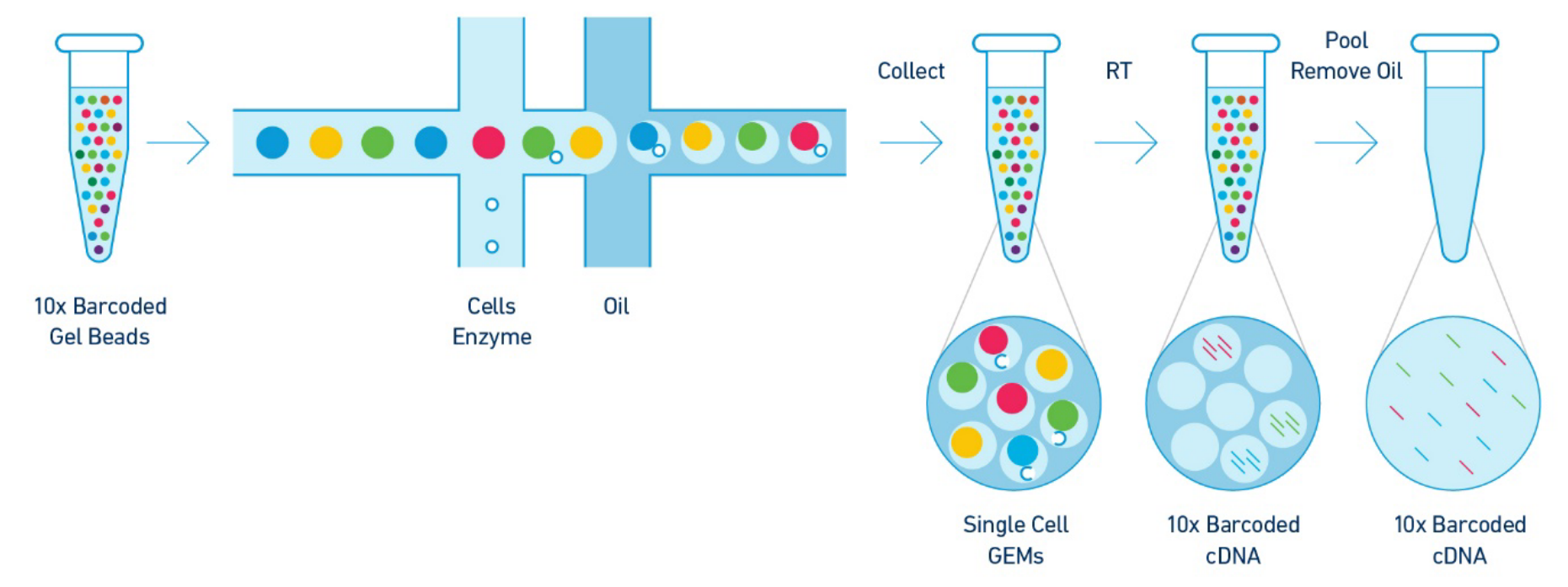 Open image in new tab
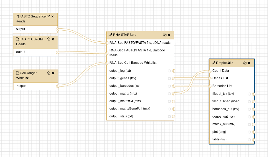 Open image in new tab
Open image in new tab


 Open image in new tab
Open image in new tab
 Open image in new tab
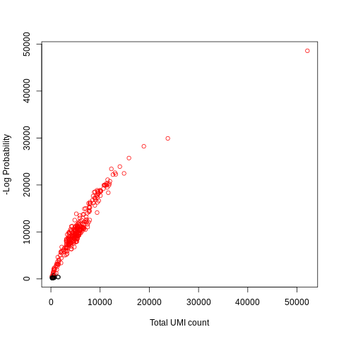 Open image in new tab