In metagenomics, information about micro-organisms in an environment can be extracted with two main techniques:
Amplicon sequencing, which sequences only the rRNA or ribosomal DNA of organisms
Shotgun sequencing, which sequences full genomes of the micro-organisms in the environment
In this tutorial, we will introduce the two main types of analyses with their general principles and differences. For a more in-depth look at these analyses, we recommend our detailed tutorials on each analysis.
We will use two datasets (one amplicon and one shotgun) from the same project on the Argentinean agricultural pampean soils. In this project, three different geographic regions that are under different types of land uses and two soil types (bulk and rhizospheric) were analyzed using shotgun and amplicon sequencing. We will focus on data from the Argentina Anguil and Pampas Bulk Soil (the original study included one more geographical regions Rascovan et al. 2013.
Amplicon sequencing is a highly targeted approach for analyzing genetic variation in specific genomic regions.
In the metagenomics fields, amplicon sequencing refers to capture and sequence of rRNA data in a sample.
It can be 16S for bacteria or archea or 18S for eukaryotes.
The highly conserved regions make it easy to target the gene across different organisms, while the highly variable regions allow us to distinguish between different species.
With amplicon data, we can determine the micro-organisms from which the sequences in our sample are coming from. This is called taxonomic assignation.
We try to assign sequences to taxons and then classify or extract the taxonomy in our sample.
In this analysis, we will use the mothur tool suite, but only a small portion of its tools and possibilities.
To learn more in detail about how to use this tool, check out the full mothur tutorial.
Importing the data
Our datasets come from a soil samples in two different Argentinian locations, for which the 16S rDNA V4 region
has been sequenced using 454 GS FLX Titanium. For the tutorial, the original fastq data has been down sampled and converted to fasta. The original data are available at EBI Metagenomics under the following run numbers:
Import the following files from Zenodo, or from the shared data library (in GTN - Material -> microbiome -> Analyses of metagenomics data - The global picture):
Click on “Training data” and then “Analyses of metagenomics data”
Select interesting file
Click on “Import selected datasets into history”
Import in a new history
As default, Galaxy takes the link as name, so rename them.
Preparing datasets
We will perform a multisample analysis with mothur. To do this, we will merge all reads into a single file,
and create a group file, indicating which reads belong to which samples.
Hands On: Prepare multisample analysis
Merge.filestool with the following parameters
“Merge” to fasta files
“Inputs” to the two sample fasta files
Make.grouptool with the following parameters
“Method to create group file” to Manually specify fasta files and group names
“Additional”: Add two elements to this repeat
First element
“fasta - Fasta to group” to SRR531818_pampa file
“group - Group name” to pampa
Second element (click on “Insert Additional”)
“fasta - Fasta to group” to SRR651839_anguil file
“group - Group name” to anguil
Comment: Note
Because we only have a small number of samples, we used the manual specification. If you have hundreds of samples this would quickly become bothersome. The solution? use a collection! To read more about collections in Galaxy, please see dedicated collections tutorial.
Have a look at the group file. It is a very simple file, it contains two columns: the first contains the read names, the second contains the group (sample) name, in our case pampa or anguil.
Optimization of files for computation
Because we are sequencing many of the same organisms, we anticipate that many of our sequences are
duplicates of each other. Because it’s computationally wasteful to align the same thing a bazillion
times, we’ll unique our sequences using the Unique.seqs command:
Hands On: Remove duplicate sequences
Unique.seqstool with the following parameters
“fasta” to the merged fasta file
“output format” to Name File
Question
How many sequences were unique? How many duplicates were removed?
19,502 unique sequences and 498 duplicates.
This can be determined from the number of lines in the fasta (or names) output, compared to the
number of lines in the fasta file before this step.
This Unique.seqs tool outputs two files: a fasta file containing only the unique sequences, and a names file.
The names file consists of two columns, the first contains the sequence names for each of the unique sequences, and the second column contains all other sequence names that are identical to the representative sequence in the first column.
name          representatives
read_name1    read_name2,read_name,read_name5,read_name11
read_name4    read_name6,read_name,read_name10
read_name7    read_name8
...
Hands On: Count sequences
Count.seqstool with the following parameters
“name” to the name file from Unique.seqs
“Use a group file” to yes
“group” to the group file from Make.group
The Count.seqs file keeps track of the number of sequences represented by each unique representative across multiple samples. We will pass this file to many of the following tools to be used or updated as needed.
Quality Control
The first step in any analysis should be to check and improve the quality of our data.
This tells us that we have a total of 19,502 unique sequences, representing 20,000 total sequences that vary in length between 80 and 275 bases. Also, note that at least some of our sequences had some ambiguous base calls.
Furthermore, at least one read had a homopolymer stretch of 31 bases, this is likely an error so we would like to filter such reads out as well.
If you are thinking that 20,000 is an oddly round number, you are correct; we downsampled the original datasets to 10,000 reads per sample for this tutorial to reduce the amount of time the analysis steps will take.
We can filter our dataset on length, base quality, and maximum homopolymer length using the Screen.seqs tool
The following tool will remove any sequences with ambiguous bases (maxambig parameter), homopolymer stretches of 9 or more bases (maxhomop parameter) and any reads longer than 275 bp or shorter than 225 bp.
Hands On: Filter reads based on quality and length
Screen.seqstool with the following parameters
“fasta” to the fasta file from Unique.seqs
“minlength” parameter to 225
“maxlength” parameter to 275
“maxambig” parameter to 0
“maxhomop” parameter to 8
“count” to the count file from Count.seqs
Question
How many reads were removed in this screening step? (Hint: run the Summary.seqs tool again)
1,804.
This can be determined by looking at the number of lines in bad.accnos output of screen.seqs step or by comparing the total number of seqs between of the summary.seqs log before and after this screening step
Sequence Alignment
Aligning our sequences to a reference helps improve OTU assignment [Schloss et. al.], so we will now align our sequences to an alignment of the V4 variable region of the 16S rRNA. This alignment has been created as described in [mothur’s MiSeq SOP] from the Silva reference database.
Between which positions most of the reads are aligned to this references?
17,698 are aligned
From this we can see that most of our reads align nicely to positions 3080-13424 on this reference. This corresponds exactly to the V4 target region of the 16S gene.
To make sure that everything overlaps the same region we’ll re-run Screen.seqs to get sequences that start at or before position 3,080 and end at or after position 13,424.
Hands On: Remove poorly aligned sequences
Screen.seqstool with the following parameters
“fasta” to the aligned fasta file
“start” to 3080
“end” to 13424
“count” to the group file created by the previous run of Screen.seqs
Question
How many sequences were removed in this step?
4,579 sequences were removed. This is the number of lines in the bad.accnos output.
Now we know our sequences overlap the same alignment coordinates, we want to make sure they only overlap that region. So we’ll filter the sequences to remove the overhangs at both ends. In addition, there are many columns in the alignment that only contain external gap characters (i.e. “.”), while columns containing only internal gap characters (i.e., “-“) are not considered. These can be pulled out without losing any information. We’ll do all this with Filter.seqs:
Hands On: Filter sequences
Filter.seqstool with the following parameters
“fasta”” to good.fasta output from Screen.seqs
“trump” to .
Extraction of taxonomic information
The main questions when analyzing amplicon data are: Which micro-organisms are present in an environmental samples? And in what proportion? What is the structure of the community of the micro-organisms?
The idea is to take the sequences and assign them to a taxon. To do that, we group (or cluster) sequences based on their similarity to defined Operational Taxonomic Units (OTUs): groups of similar sequences that can be treated as a single “genus” or “species” (depending on the clustering threshold)
Comment: Background: Operational Taxonomic Units (OTUs)
In 16S metagenomics approaches, OTUs are clusters of similar sequence variants of the 16S rDNA marker gene sequence. Each of these clusters is intended to represent a taxonomic unit of a bacterial species or genus depending on the sequence similarity threshold. Typically, OTU clusters are defined by a 97% identity threshold of the 16S gene sequence variants at genus level. 98% or 99% identity is suggested for species separation.
Figure 4: Cladogram of operational taxonomic units (OTUs). Credit: Danzeisen et al. 2013, 10.7717/peerj.237
The first thing we want to do is to further de-noise our sequences from potential sequencing errors, by pre-clustering the sequences using the Pre.cluster command, allowing for up to 2 differences between sequences. This command will split the sequences by group and then sort them by abundance, then go from most abundant to least and identify sequences that differ by no more than 2 nucleotides from on another. If this is the case, then they get merged. We generally recommend allowing 1 difference for every 100 basepairs of sequence:
Hands On: Perform preliminary clustering of sequences and remove undesired sequences
Pre.clustertool with the following parameters
“fasta” to the fasta output from the last Filter.seqs run
“name file or count table” to the count table from the last Screen.seqs step
“diffs” to 2
Question
How many unique sequences are we left with after this clustering of highly similar sequences?
10,398
This is the number of lines in the fasta output
We would like to classify the sequences using a training set, which is again is provided on [mothur’s MiSeq SOP].
Hands On: Classify the sequences into phylotypes
Import the trainset16_022016.pds.fasta and trainset16_022016.pds.tax in your history
You will see that every read now has a classification.
The next step is to use this information to determine the abundances of the different found taxa. This consists of three steps:
first, all individual sequences are classified, and get assigned a confidence score (0-100%)
next, sequences are grouped at 97% identity threshold (not using taxonomy info)
finally, for each cluster, a consensus classification is determined based on the classification of the individual sequences and taking their confidence scores into account
Hands On: Assign sequences to OTUs
Cluster.splittool with the following parameters
“Split by” to Classification using fasta
“fasta” to the fasta output from Pre.cluster
“taxonomy” to the taxonomy output from Classify.seqs
“count” to the count table output from Pre.cluster
“Clustering method” to Average Neighbour
“cutoff” to 0.15
We obtain a table with the columns being the different identified OTUs, the rows the different distances and the cells the ids of the sequences identified for these OTUs for the different distances.
Next we want to know how many sequences are in each OTU from each group with a distance of 0.03 (97% similarity). We can do this using the Make.shared command with the 0.03 cutoff level:
Hands On: Estimate OTU abundance
Make.sharedtool with the following parameters
“Select input type” to OTU list
“list” to list output from Cluster.split
“name file or count table” to the count table from Pre.cluster
“label” to 0.03
We probably also want to know the taxonomy for each of our OTUs. We can get the consensus taxonomy for each OTU using the Classify.otu command:
Hands On: Classify the OTUs
Classify.otutool with the following parameters
“list” to output from Cluster.split
“count” to the count table from Pre.cluster
“Select Taxonomy from” to History
“taxonomy” to the taxonomy output from Classify.seqs
“label” to 0.03
Question
How many OTUs with taxonomic assignation are found for the Anguil sample? And for the Pampa sample?
What is the annotation of first OTU and its size?
2,195 for Anguil and 2,472 for Pampa (“tax.summary”)
Otu00001 is associated to 929 sequences and to Bacteria (kingdom), Verrucomicrobia (phylum), Spartobacteria (class) in “taxonomy” file
Visualization
We have now determined our OTUs and classified them, but looking at a long text file is not very informative.
Let’s visualize our data using Krona:
Hands On: Krona
First we convert our mothur taxonomy file to a format compatible with Krona
Taxonomy-to-Kronatool with the following parameters
“Taxonomy file” to the taxonomy output from Classify.otu (note: this is a collection input)
Krona pie charttool with the following parameters
“Type of input” to Tabular
“Input file” to taxonomy output from Taxonomy-to-Krona (collection)
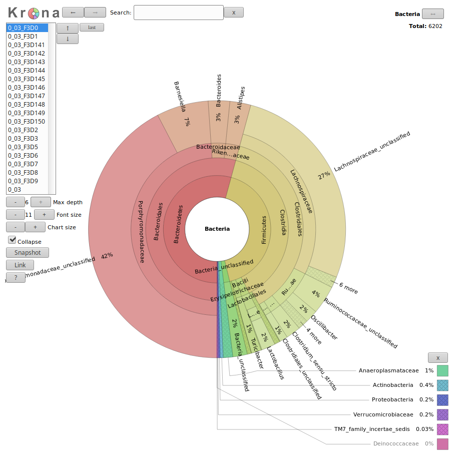
The result is an HTML file with an interactive visualization, for instance try clicking
on one of the rings in the image or playing around with some of the settings.
This produced a single plot for both your samples, but what if you want to compare
the two samples?
Hands On: Per-sample Krona plots
Classify.otutool
Hit the rerun button on the Classify.otu job in your history and see if you can find settings that will give you per-sample taxonomy data
Kronatool
Now use this new output collection to create per-sample Krona plots
In this new Krona output you can switch between the combined plot and the per-sample plots via the selector in the top-left corner.
Question
Which soil sample had a higher percentage of Acidobacteria, anguil or pampa? what were the respective percentages?
The anguil sample had a higher proportion of Acidobacteria. The exact percentages can be found by looking at the pie charts at the
top right-hand corner after clicking on the label Acidobacteria. For anguil the percentage is 36%, for the pampa sample it is 26%.
To further explore the community structure, we can visualize it with dedicated tools such as Phinch.
Hands On: Visualization of the community structure with Phinch
Make.biomtool with the following parameters
“shared” to Make.shared output
“constaxonomy” to taxonomy output from the first run of Classify.otu (collection)
Expand the dataset and click on the “view biom at phinch” link
Comment
If this link is not present on your Galaxy, you can download the generated BIOM file and upload directly to Phinch server at http://phinch.org.
Once we have information about the community structure (OTUs with taxonomic structure), we can do more analysis on it: estimation of the diversity of micro-organism, comparison of diversity between samples, analysis of populations, … We will not go into detail of such analyses here but you can follow our tutorials on amplicon data analyses to learn more about them.
Shotgun metagenomics data
In the previous section, we saw how to analyze amplicon data to extract the community structure. Such information can also be extracted from shotgun metagenomic data.
In shotgun data, full genomes of the micro-organisms in the environment are sequenced (not only the 16S or 18S). We can then have access to the rRNA (only a small part of the genomes), but also to the other genes of the micro-organisms. Using this information, we can try to answer questions such as “What are the micro-organisms doing?” in addition to the question “What micro-organisms are present?”.
In this second part, we will use a metagenomic sample of the Pampas Soil (SRR606451).
Data upload
Hands On: Data upload
Create a new history
Import the SRR606451_pampa Fasta file from Zenodo or from the data library (in “Analyses of metagenomics data”)
As for amplicon data, we can extract taxonomic and community structure information from shotgun data. Different approaches can be used:
Same approach as for amplicon data with identification and classification of OTUs
Such an approach requires a first step of sequence sorting to extract only the 16S and 18S sequences, then using the same tools as for amplicon data. However, rRNA sequences represent a low proportion (< 1%) of the shotgun sequences so such an approach is not the most statistically supported
Assignation of taxonomy on the whole sequences using databases with marker genes
In this tutorial, we use the second approach with MetaPhlAn2. This tools is using a database of ~1M unique clade-specific marker genes (not only the rRNA genes) identified from ~17,000 reference (bacterial, archeal, viral and eukaryotic) genomes.
Hands On: Taxonomic assignation with MetaPhlAn2
MetaPhlAN2tool with
“Input file” to the imported file
“Database with clade-specific marker genes” to locally cached
“Cached database with clade-specific marker genes” to MetaPhlAn2 clade-specific marker genes
Each line contains a taxa and its relative abundance found for our sample. The file starts with high level taxa (kingdom: k__) and go to more precise taxa.
A BIOM file with the same information as the previous file but in BIOM format
It can be used then by mothur and other tools requiring community structure information in BIOM format
A SAM file with the results of the mapping of the sequences on the reference database
Question
What is the most precise level we have access to with MetaPhlAn2?
What are the two orders found in our sample?
What is the most abundant family in our sample?
We have access to species level
Pseudomonadales and Solirubrobacterales are found in our sample
The most abundant family is Pseudomonadaceae with 86.21 % of the assigned sequences
Even if the output of MetaPhlAn2 is bit easier to parse than the BIOM file, we want to visualize and explore the community structure with KRONA
Hands On: Interactive visualization with KRONA
Format MetaPhlAn2 output for Kronatool with
“Input file” to Community profile output of MetaPhlAn2
KRONA pie charttool with
“What is the type of your input data” as MetaPhlan
“Input file” to the output of Format MetaPhlAn2
Extraction of functional information
We would now like to answer the question “What are the micro-organisms doing?” or “Which functions are performed by the micro-organisms in the environment?”.
In the shotgun data, we have access to the gene sequences from the full genome. We use that to identify the genes, associate them with a function, build pathways, etc., to investigate the functional part of the community.
Hands On: Metabolism function identification
HUMAnN2tool with
“Input sequence file” to the imported sequence file
“Use of a custom taxonomic profile” to Yes
“Taxonomic profile file” to Community profile output of MetaPhlAn2
“Nucleotide database” to Locally cached
“Nucleotide database” to Full
“Protein database” to Locally cached
“Protein database” to Full UniRef50
“Search for uniref50 or uniref90 gene families?” to uniref50
“Database to use for pathway computations” to MetaCyc
“Advanced Options”
“Remove stratification from output” to Yes
This step is long so we generated the output for you!
Import the 3 files whose the name is starting with “humann2”
Gene family abundance is reported in RPK (reads per kilobase) units to normalize for gene length. It reflects the relative gene (or transcript) copy number in the community.
The “UNMAPPED” value is the total number of reads which remain unmapped after both alignment steps (nucleotide and translated search). Since other gene features in the table are quantified in RPK units, “UNMAPPED” can be interpreted as a single unknown gene of length 1 kilobase recruiting all reads that failed to map to known sequences.
A file with the coverage of pathways
Pathway coverage provides an alternative description of the presence (1) and absence (0) of pathways in a community, independent of their quantitative abundance.
A file with the abundance of pathways
Question
How many gene families and pathways have been identified?
44 gene families but no pathways are identified
The RPK for the gene families are quite difficult to interpret in term of relative abundance. We decide then to normalize the values
Hands On: Normalize the gene family abundances
Renormalize a HUMAnN2 generated tabletool with
“Gene/pathway table” to the gene family table generated with HUMAnN2
“Normalization scheme” to Relative abundance
“Normalization level” to Normalization of all levels by community total
Question
What percentage of sequences has not be assigned to a gene family?
What is the most abundant gene family?
55% of the sequences have not be assigned to a gene family
The most abundant gene family with 25% of sequences is a putative secreted protein
With the previous analyses, we investigate “Which micro-organims are present in my sample?” and “What function are performed by the micro-organisms in my sample?”. We can go further in these analyses (for example, with a combination of functional and taxonomic results). We did not detail that in this tutorial but you can find more analyses in our tutorials on shotgun metagenomic data analyses.
Conclusion
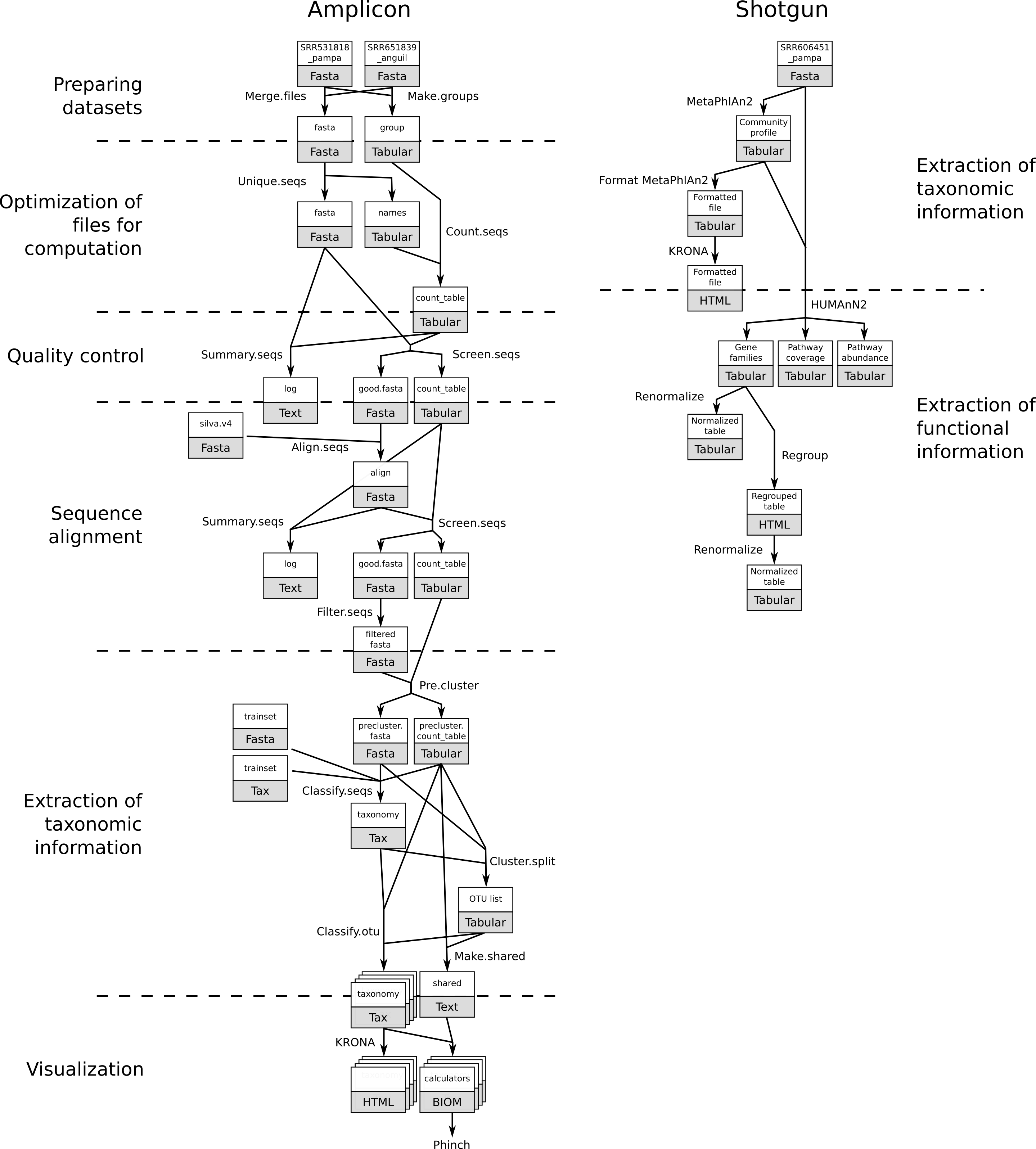
We can summarize the analyses with amplicon and shotgun metagenomic data:
Both analyses are quite complex! However, in this tutorial, we only showed simple cases of metagenomics data analysis with subset of real data.
Check our other tutorials to learn more in detail of how to analyze metagenomics data.
You've Finished the Tutorial
Please also consider filling out the Feedback Form as well!
Key points
With amplicon data, we can extract information about the studied community structure
With shotgun data, we can extract information about the studied community structure and also the functions realised by the community
The tools used to analyze amplicon and shotgun data are different, except for the visualisation
Metagenomics data analyses are complex and time-consuming
Frequently Asked Questions
Have questions about this tutorial? Have a look at the available FAQ pages and support channels
Further information, including links to documentation and original publications, regarding the tools, analysis techniques and the interpretation of results described in this tutorial can be found here.
References
Rascovan, N., B. Carbonetto, S. Revale, M. D. Reinert, R. Alvarez et al., 2013 The PAMPA datasets: a metagenomic survey of microbial communities in Argentinean pampean soils. Microbiome 1: 10.1186/2049-2618-1-21
Feedback
Did you use this material as an instructor? Feel free to give us feedback on how it went.
Did you use this material as a learner or student? Click the form below to leave feedback.
Hiltemann, Saskia, Rasche, Helena et al., 2023 Galaxy Training: A Powerful Framework for Teaching! PLOS Computational Biology 10.1371/journal.pcbi.1010752
Batut et al., 2018 Community-Driven Data Analysis Training for Biology Cell Systems 10.1016/j.cels.2018.05.012
@misc{microbiome-general-tutorial,
author = "Saskia Hiltemann and Bérénice Batut",
	title = "Analyses of metagenomics data - The global picture (Galaxy Training Materials)",
	year = "",
	month = "",
	day = "",
	url = "\url{https://training.galaxyproject.org/training-material/topics/microbiome/tutorials/general-tutorial/tutorial.html}",
	note = "[Online; accessed TODAY]"
}
@article{Hiltemann_2023,
	doi = {10.1371/journal.pcbi.1010752},
	url = {https://doi.org/10.1371%2Fjournal.pcbi.1010752},
	year = 2023,
	month = {jan},
	publisher = {Public Library of Science ({PLoS})},
	volume = {19},
	number = {1},
	pages = {e1010752},
	author = {Saskia Hiltemann and Helena Rasche and Simon Gladman and Hans-Rudolf Hotz and Delphine Larivi{\`{e}}re and Daniel Blankenberg and Pratik D. Jagtap and Thomas Wollmann and Anthony Bretaudeau and Nadia Gou{\'{e}} and Timothy J. Griffin and Coline Royaux and Yvan Le Bras and Subina Mehta and Anna Syme and Frederik Coppens and Bert Droesbeke and Nicola Soranzo and Wendi Bacon and Fotis Psomopoulos and Crist{\'{o}}bal Gallardo-Alba and John Davis and Melanie Christine Föll and Matthias Fahrner and Maria A. Doyle and Beatriz Serrano-Solano and Anne Claire Fouilloux and Peter van Heusden and Wolfgang Maier and Dave Clements and Florian Heyl and Björn Grüning and B{\'{e}}r{\'{e}}nice Batut and},
	editor = {Francis Ouellette},
	title = {Galaxy Training: A powerful framework for teaching!},
	journal = {PLoS Comput Biol}
}
Congratulations on successfully completing this tutorial!
You can use Ephemeris's shed-tools install command to install the tools used in this tutorial.
4 stars:
Liked: Structure of the content
Disliked: Nothing to say
5 stars:
Liked: Detailed guidance
Disliked: 1. The visualisation step using Phinch did not work properly for me in the Galaxy. I don't know why but the step is still running (marked in yellow) even after a day. No problem, because I run it using the software. 2. During the visualisation using Amplicon data, when I had to re-run the Classify.otu after the 1st Krona pie chart, the number of samples was supposed to drop down or something similar (or in the Extraction of Taxonomic Information step, I am slightly mixing them up). By following the exact steps, I could not regenerate the same.
May 2024
5 stars:
Disliked: Usegalaxy.org did not support the metaplAN2 and HUManN2.
November 2022
5 stars:
Liked: Hands in
Disliked: Videos might help us more
4 stars:
Liked: well described
Disliked: help when stuck
December 2019
5 stars:
Liked: flow of the tutorial
Disliked: more accurate galaxy functions reference.
April 2019
4 stars:
Liked: step by step very well described
Disliked: data analysis with OTU / phylotype
November 2018
4 stars:
Liked: clear step by step module
4 stars:
Liked: The overview of all the tools available.
Disliked: The time for the processes on Galaxy.
October 2018
1 stars:
Liked: Some instructions were not clear at all, please be more specific as i encounter errors very likely despite following the steps
Disliked: Please review the protocol and revise some segments
2 stars:
Liked: Krona
Disliked: It needs to be updated, some returns error and some is missing. Be more detail and specific
Questions:
Open image in new tab
Open image in new tab
Open image in new tab
Open image in new tab
Open image in new tab