Tree thinking for tuberculosis evolution and epidemiology
| Author(s) |
|
| Editor(s) |
|
| Reviewers |
|
OverviewQuestions:
Objectives:
What information can I get from a phylogenetic tree?
How do I estimate a phylogeny?
Requirements:
Understand the basic concepts behind phylogenetic trees, as applied to Mycobacterium tuberculosis
Be able to read and interrogate a phylogeny encountered in the literature
- Introduction to Galaxy Analyses
- tutorial Hands-on: M. tuberculosis Variant Analysis
- tutorial Hands-on: Identifying tuberculosis transmission links: from SNPs to transmission clusters
Time estimation: 1 hourLevel: Introductory IntroductorySupporting Materials:Published: Mar 16, 2022Last modification: Jun 4, 2025License: Tutorial Content is licensed under Creative Commons Attribution 4.0 International License. The GTN Framework is licensed under MITpurl PURL: https://gxy.io/GTN:T00144rating Rating: 5.0 (1 recent ratings, 11 all time)version Revision: 12
“Nothing in biology makes sense except in the light of evolution.”
Phylogenetic trees are a tool for organizing biological diversity. Just as maps provide a spatial framework to the geographer, phylogenies provide an evolutionary context to the biologist: they capture the relationship among “things” (species, individuals, genes), represented as tips in the tree, based on common ancestry.
In evolutionary and epidemiological studies of Mycobacterium tuberculosis, it is now common to encounter large phylogenetic trees. Being able to read and critically examine them is extremely useful. Phylogenies can be used to understand the origin of a disease or the onset of an epidemic, to distinguish ongoing transmission from imported cases, to investigate how specific traits like antibiotic resistance evolve et cetera et cetera. Many research ideas originate from looking at and discussing patterns present in phylogenies.
This tutorial provides an introduction to phylogenetic trees in the context of whole genome sequencing of Mycobacterium tuberculosis strains. Phylogenetics is a vast topic, and we can only scratch its surface here. For those motivated to delve deeper into the topic, the Resources section contains links and reading suggestions.
Basic concepts: How to read a phylogeny
Below are two phylogenies of the Mycobacterium tuberculosis complex (MTBC) to illustrate some basic vocabulary and concepts.
If the following discussion sounds a bit too esoteric, you might be interested in a more thorough introduction to the topic of phylogeny like provided, for example, by the introduction to phylogenetics from the EMBL-EBI collection of online tutorials.
Rooted trees and tree topology
The trees in figure 1 look rather different at a first glance, but they are identical except for one key aspect: tree A is rooted while tree B is not.
What is the difference between the two? First, let’s state what is the same in the two trees: the tree topology, that is, the relative branching order. The same groupings are present in the two trees: they both contain the same information about the relatedness of strains. An example: TB isolated from Peruvian mummies is most similar to M. pinnipedii known from marine mammals; they share a most recent common ancestor. This can be seen in the rooted as well as in the unrooted tree.
The key difference between the rooted and the unrooted tree is that only the rooted tree shows the direction and sequence of branching events. The unrooted tree does not tell us, for example, whether M. bovis diverged early or late in the history of the MTBC. It is thus compatible with the old hypothesis that human TB evolved from animal TB. The rooted tree shows that this hypothesis is most likely wrong: animal-associated strains are not ancestral to human-associated strains.
The best way to root a tree is by including an outgroup: a species or lineage which we know a priori to lay outside the phylogeny we’re interested in. M. canettii usually serves this purpose for studying the MTBC, but you can also root, for example, a phylogeny of lineage 2 by including a lineage 4 strain.
Branch lengths
Besides relatedness and direction, a third important piece of information contained in a phylogeny is the branch length. When a phylogeny has been estimated from DNA or protein sequences, branch lengths usually reflect the evolutionary distance between nodes in the tree. This information can be used to translate distance in terms of expected nucleotide changes into years, and thus to connect evolutionary change to historical events.
 Open image in new tab
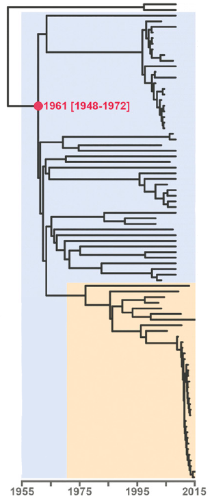
As branch lengths reflect evolutionary distances, they can also be used to identify transmission clusters and outbreaks. Figure 2 shows a (rooted) tree of the Central Asian Clade (CAC), which is part of lineage 2 (Eldholm et al. 2016). The orange color highlights the Afghan strain family within the CAC. At the bottom of the tree, note the clade with short branch lengths. This is how one would expect an outbreak to look in a phylogenetic tree: a set of strains clustering together and separated by extremely short branches, reflecting their almost identical genomes.
Comment: Phylogenetics with Mycobacterium tuberculosisPhylogenetics with MTB has some particularities rarely encountered with other organisms.
There seems to be no horizontal gene transfer (HGT) in the MTBC. HGT complicates phylogenetic inference in many bacteria because a piece of DNA introduced by HGT has a different history and thus phylogeny than genes not affected by HGT.
There is little genetic diversity in the MTBC: any two strains differ by only around 2,500 SNPs over the whole genome. To achieve a good resolution of recent evolution (e.g. during an outbreak), whole genome sequences are thus extremely useful.
A large proportion of DNA polymorphisms in the MTBC are singletons, that is, variants present only in a single strain. This adds to the problem of low diversity, since singletons are not informative about tree topology.
In this workshop, and indeed in many studies of the MTBC, SNPs are called not against the reference strain H37Rv, but against a reconstructed ancestral genome. This means that the number of SNPs identified does not reflect the evolutionary distance from some random strain like H37Rv, but from the most recent common ancestor of the MTBC. Take a look at Figure 3 in Goig et al. 2018 to see how this affects the number of SNPs identified in a genome. Below we will see that this has implications for the interpretation of a tree.
Infering phylogeny from SNP alignments
Aligned DNA or protein sequences are the starting material for phylogenetic inference with molecular data.
In this tutorial we will explore the phylogenetic relationship between 19 MTBC strains and 1 strain of M. canettii, where the latter is included as outgroup, allowing us to root the phylogeny. Our starting point will be an alignment of all SNPs identified from whole-genome sequencing data of these 20 strains. This SNP alignment was generated by
- mapping short sequenced reads from each sample to the infered sequence of the most recent common ancestor of the MTBC as the reference
- calling variants against that reference from the mapped reads of each sample
- incorporating the SNP variants of each sample into the reference to obtain a consensus genome of that sample
- combining the consensus genomes into a single multi-sequence fasta dataset
- discarding bases found to be identical in all samples from all sequences
Comment: Recommended tutorialsSteps 1 and 2 are explained in detail in the tutorial MTB variant analysis. Steps 3 - 5 are conducted for the exact same 20 samples used here in the tutorial on transmission clusters.
If you want to gain a complete understanding of the whole process of sequencing-based analysis of MTBC strains, we recommend you, if you have not done so yet, to work through these two tutorials in the order above before continuing with this one here.
Figure 3 shows a snapshot of an illustrative SNP alignment. Each row in the alignment represents a different strain, each column a position in the reference genome.
 Open image in new tab
Because this alignment is based on SNPs, it contains only variable positions. This is important to keep in mind! Genetic distances between strains will be hugely overestimated if we leave out all the positions which show no variation!
Near the end of this tutorial, we will show and discuss ways to correct for this.
Comment: The alternative approach: genome assemblyA frequently used alternative approach to obtain a phylogeny from short read data is to a) assemble the genomes (see the numerous Galaxy tutorials on this topic), b) annotate genes, c) extract genes present in all strains (the “core” genes), d) align the core genes. This approach underlies core genome multilocus sequence typing (cgMLST), which is often used to genotype bacterial pathogens (e.g. Zhou et al. 2021).
With this bit of introduction you should, hopefully, be prepared to follow the flow and purpose of the analysis presented here.
AgendaIn this tutorial, we will cover:
Phylogenetic analysis of MTBC strains with Galaxy and Rstudio
Get the data
If you have worked at least through the first part of the tutorial on transmission clusters before coming here, you are all set.
You can continue working in the same history you created for the other tutorial, or copy the SNP alignment (the output of Finds SNP sites tool) over to a new one, and can safely skip the following first hands-on part.
If you are not interested in that other tutorial, here are the instructions for setting up a history for the analysis here, and for obtaining a copy of the SNP alignment from Zenodo.
Hands On: Create a new history and prepare the input data
Create a new history for this analysis
To create a new history simply click the new-history icon at the top of the history panel:
Give the history a suitable name
- Click on galaxy-pencil (Edit) next to the history name (which by default is “Unnamed history”)
- Type the new name:
MTB tree thinking tutorial- Click on Save
- To cancel renaming, click the galaxy-undo “Cancel” button
If you do not have the galaxy-pencil (Edit) next to the history name (which can be the case if you are using an older version of Galaxy) do the following:
- Click on Unnamed history (or the current name of the history) (Click to rename history) at the top of your history panel
- Type the new name:
MTB tree thinking tutorial- Press Enter
Upload a version of the SNP alignment via this URL
https://zenodo.org/record/6010176/files/SNP_alignment.fastaand make sure the dataset format is set to
fasta.
- Copy the link location
Click galaxy-upload Upload at the top of the activity panel
- Select galaxy-wf-edit Paste/Fetch Data
Paste the link(s) into the text field
Change Type (set all): from “Auto-detect” to
fastaPress Start
- Close the window
Replace Text in entire line ( Galaxy version 1.1.2) to clean up the aligned sequence names
- param-file “File to process”: the uploaded SNP alignment
- In param-repeat “1. Replacement”:
- “Find pattern”:
^(>.+)\.fastq.*- “Replace with”:
\1From just a brief inspection of the downloaded SNP alignment, you should see that the sequence names in that file carry a
.fastq.vcfor.fastq.gz.vcfsuffix on the actual sample names. The above replacement operation, drops these unnecessary endings, which we would otherwise carry over to all outputs generated in the analysis.When the Replace Text tool run is finished, rename the output dataset to, for example, SNP alignment
- Click on the galaxy-pencil pencil icon for the dataset to edit its attributes
- In the central panel, change the Name field to
SNP alignment- Click the Save button
Take a look at the alignment
Click on the dataset that you just renamed to expand it in the history, then click on galaxy-barchart Visualize and try both, the “Editor” and the “Multiple Sequence Alignment”.
Can you see one of the MTBC particularities mentioned above, the predominance of singletons?
How many sites are there in the alignment?
Also take a look at the M. canettii sequence: being the outgroup, it has a large number of SNPs.


Set up the coding environment
We will use R to estimate a tree from a nucleotide alignment and to plot and manipulate the tree. We will provide you with the exact code to produce the figures we need, and, conveniently, you can run this code from an RStudio session that you can start as an interactive tool inside Galaxy.
If you have worked with R or RStudio previously, feel free to use any kind of coding environment for exploring and manipulating the tree - just download it from your history and import it into any R session you have access to.
Hands On: Starting an RStudio session and setting things up
Note the dataset number (the number in front of and separated with a : from the dataset name) of the file called “SNP_alignment.fasta”
Run RStudio
Hands On: Launch RStudioDepending on which server you are using, you may be able to run RStudio directly in Galaxy. If that is not available, RStudio Cloud can be an alternative.
Currently RStudio in Galaxy is only available on UseGalaxy.eu and UseGalaxy.org
- Open the Rstudio tool tool by clicking here to launch RStudio
- Click Run Tool
- The tool will start running and will stay running permanently
- Click on the “User” menu at the top and go to “Active InteractiveTools” and locate the RStudio instance you started.
If RStudio is not available on the Galaxy instance:
- Register for RStudio Cloud, or login if you already have an account
- Create a new project
- Install and use the ape R package
- Click on the Terminal tab (at the top of the Rstudio window)
Execute the command:
conda install r-apeThis will install the ape package into the environment of the running session.
When the previous step has finished, switch back to the Console tab and run the command
library("ape")You might get a warning about R versions, which you can ignore.
Import the SNP alignment into the Rstudio session
alignment_file <- gx_get(###)where you have to replace
###with the dataset number of the alignment file in your history.
Estimate the tree
We have now set up our R session and are ready to start. As a first step we would like to load the alignment into R and infer a tree from it.
In this tutorial, we’ll use the neighbor-joining algorithm to estimate a phylogenetic tree for the 20 strains. The details of how these methods construct trees from an alignment are beyond the scope of this introductory course. To be able to read trees, it is not necessary to know the statistical and computational details of how the trees are estimated. The books listed in the Resources section provide in-depth introductions into the different principles of phylogenetic inference, in particular Baum & Smith 2013 and Yang 2014.
CommentIf you are experienced with R, you are encouraged also to start playing with all the code from here on, to modify it, and to explore the numerous phylogenetics packages and functions available in R.
Hands On: Estimate a phylogeny and plot it# Load the alignment aln <- read.dna(alignment_file, format="fasta") # Remove the ugly file extensions from the sample names rownames(aln) <- gsub('.fastq.vcf', '', rownames(aln)) rownames(aln) <- gsub('.fastq.gz.vcf', '', rownames(aln)) # Estimate a distance matrix, showing how many nucleotide differences there are between any two samples dmat <- dist.dna(aln, model='N') # Infer the tree from the matrix using neighbor-joining tree <- nj(dmat) # Plot the tree plot(tree)Question
- Take a look at the tree. Is it rooted or unrooted? What is the strain far apart from all other strains?
- The tree is unrooted, and the outlier strain is M. canettii, our outgroup. The much longer branch leading to this strain shows that many SNPs separate M. canettii from the common ancestor of the MTBC.

Root the tree
Phylogenetic trees are great tools because they are at the same time quantitative (we can do calculations on branch lengths, estimate uncertainty of a tree topology etc.) and visually appealing, allowing to actually “see” biologically interesting patterns. Often this requires some tweaking of the tree, for example by coloring parts of the tree according to some background information we have about the samples.
To make the phylogeny more interpretable, we will now root the tree using the M. canettii strain as the outgroup, then exclude that strain, such that patterns within the MTBC become clearer.
Hands On: Root the tree and drop its outgroup# Root the tree tree_rooted <- root(tree, "ERR313115") # Remove the outgroup to make distances within MTB clearer tree_rooted <- drop.tip(tree_rooted, "ERR313115") tree_rooted$root.edge <- 0.005 plot(tree_rooted, root.edge = T, cex=0.6)

This already looks better, the tree topology stands out more clearly now, and we can identify groups of closely related strains.
Create tree with lineage as tip label instead of strain name
A first piece of information we now want to add to the phylogeny is to which lineage the strains belong. This will allow us to assess whether our tree is consistent with the known phylogeny of the MTBC, shown in Figure 1A, and to visualize which lineages are present in our sample. The information to which lineage a strain belongs can be found in the output of TB-profiler, as explained in the tutorial on TB variant analysis.
Hands On: Generate a tree with lineage labels# Assign lineages to samples, as identified by TB-profiler mtbc_lineages <- c( "ERR181435" = "L7", "ERR313115" = "canettii", "ERR551620" = "L5", "ERR1203059" = "L5", "ERR2659153" = "orygis", "ERR2704678" = "L3", "ERR2704679" = "L1", "ERR2704687" = "L6", "ERR5987300" = "L2", "ERR5987352" = "L4", "ERR6362078" = "L2", "ERR6362138" = "L2", "ERR6362139" = "L4", "ERR6362156" = "L2", "ERR6362253" = "L2", "ERR6362333" = "L2", "ERR6362484" = "L4", "ERR6362653" = "L2", "SRR998584" = "L5", "SRR13046689" = "bovis" ) # Replace the tree labels tree_lineages <- tree_rooted tree_lineages$tip.label <- as.character(mtbc_lineages[tree_rooted$tip.label]) # Define some colors for the lineages color_code_lineages = c( L1 = "#ff00ff", L2 = "#0000ff", L3 = "#a000cc", L4 = "#ff0000", L5 = "#663200", L6 = "#00cc33", L7 = "#ede72e", bovis="black", orygis="black") pal_lineages <- as.character(color_code_lineages[tree_lineages$tip.label]) # Plot the old and new tree version next to each other par(mfrow = c(1, 2)) plot(tree_rooted,cex = 0.7, root.edge = TRUE) plot(tree_lineages,cex = 0.8, tip.color = pal_lineages, root.edge = TRUE)QuestionLooking at the different lineages present in the tree, does our phylogeny make sense? Or asked differently: does our phylogeny show the same branching patterns between lineages as the established phylogeny in Fig. 1A?
There is indeed a problem with our phylogeny: one L2 and one L5 strain do not cluster with the other strains of these lineages. Instead, they appear near the root of the tree, with very short (ERR5987300) to non-existent (ERR1203059) branches. Other parts of the tree are consistent with Fig. 1A, suggesting that we can focus our first round of troubleshooting on these two strains.

First round of exercises
Question: Exercise 1An important part of bioinformatics consists in trying to find out whether a surprising observation has biological significance — or reflects a mistake somewhere in the numerous steps leading to the result. Have we just discovered two new lineages of MTB, or did we commit a stupid mistake? To find out, take a look a the TB-profiler and the VCF files for the two strange strains, which should be present in your Galaxy history if you’ve followed the previous tutorial. Compare them with “normal” strains. Do you notice something?
The VCF files hold an important hint to explain our puzzling observation: ERR1203059.vcf contains not a single SNP, ERR5987300.vcf only 81 SNPs. By contrast, the other strains have between 750 and 1250 SNPs. What happened here? To find out, we would have to take a closer look at the steps leading from BAM to VCF files. One possibility is that the sequencing depth for these samples was so low that most SNPs were filtered out because they did not pass the quality filtering.
Question: Exercise 2In the tutorial on transmission clusters two clusters of samples got identified and are reproduced below. How do these clusters show up in the phylogenetic tree? What additional information does the tree contain?
Sample Cluster_id DR profile Clustering ERR5987352 10 Pre-MDR Clustered ERR6362484 10 Pre-MDR Clustered ERR6362138 12 MDR Clustered ERR6362156 12 Pre-XDR Clustered ERR6362253 12 MDR Clustered Clusters 10 and 12 appear as clades of closely related strains in the phylogeny: cluster 12 being part of lineage 2, cluster 10 of lineage 4. The phylogeny additionally reveals that cluster 12 is part of a larger clade of rather closely related lineage 2 strains. While clustering with a fixed SNP threshold produces a binary outcome (clustered/unclustered), the phylogeny reveals the gradual nature of relatedness. With a more permissive SNP threshold for clustering, or a different pipeline to call SNPs, we might well identify a larger cluster of L2 strains.
Map a trait onto the tree
Phylogenies are particularly useful when combined with additional information. For our 19 MTB strains, for example, we might know such things as the country of origin, the sampling date, or various phenotypes determined in the lab, for example the virulence of the strains in an animal model. By mapping this additional information onto the phylogeny, we can gain insights into how, where and when these traits evolved.
For our 20 samples, a trait you previously identified (if you have been doing the tutorial on transmission clusters, is the DR profile. Let us map this trait onto the tree and see if we can learn something from the observed patterns.
Hands On: Generate a tree with DR profiles as labels# Same as before, but with DR profiles instead of lineages mtbc_dr <- c( "ERR181435" = "Sensitive", "ERR313115" = "Sensitive", "ERR551620" = "MDR", "ERR1203059" = "Sensitive", "ERR2659153" = "Sensitive", "ERR2704678" = "Sensitive", "ERR2704679" = "Sensitive", "ERR2704687" = "Sensitive", "ERR5987300" = "PreXDR", "ERR5987352" = "PreMDR", "ERR6362078" = "MDR", "ERR6362138" = "MDR", "ERR6362139" = "PreMDR", "ERR6362156" = "PreXDR", "ERR6362253" = "MDR", "ERR6362333" = "PreXDR", "ERR6362484" = "PreMDR", "ERR6362653" = "MDR", "SRR998584" = "Sensitive", "SRR13046689" = "Other" ) tree_dr <- tree_rooted tree_dr$tip.label <- as.character(mtbc_dr[tree_rooted$tip.label]) color_code_dr = c( Sensitive = "#ff00ff", PreXDR = "#0000ff", PreMDR = "#a000cc", MDR = "#ff0000", Other = "#663200" ) pal_dr <- as.character(color_code_dr[tree_dr$tip.label]) par(mfrow = c(1, 2)) plot(tree_rooted,cex = 0.7, root.edge = TRUE) plot(tree_dr,cex = 0.8, tip.color = pal_dr, root.edge = TRUE)
Exercises continued
Question: Exercise 3In the previous tutorial on clustering, you have come across the hypothesis that unclustered cases of DR represent de novo evolution of DR, while clustered cases of DR represent instances of DR transmission. Looking at lineage 2 in the phylogeny above, does this hypothesis hold? How many times would MDR have evolved independently in lineage 2? Is there an alternative explanation for the prevalence of MDR in lineage 2?
MDR would have evolved three times according to the clustering perspective mentioned above: once in cluster 12, once in ERR6362078, and once in ERR6362653. The phylogeny suggest a simpler alternative: MDR could have been already present in the common ancestor of the six L2 strains in our sample; it could have evolved only once, along the long branch leading from the split from lineage 3 to the most recent common ancestor of the six samples. This picture, however, might change with a more extensive sampling of lineage 2. Six samples are hardly sufficient to make claims about the prevalence and evolution of MDR in lineage 2. As for the interpretation of clustering, sampling design is crucial for the interpretation of phylogenies and should always be kept in mind in order to avoid overinterpretation.

Bootstrapping
Before drawing big conclusions from our tree, let us get an idea of how robust it actually is.
Bootstrapping is a resampling approach that allows us to do that. The basic idea is that we draw sites randomly from our original alignment, and from this “artifical alignment” we estimate a tree. We repeat this procedure 100 times and then ask how many times the same nodes occur in the bootstrap trees. All these steps are conveniently implemented in ape’s boot.phylo() function.
Hands On: Get bootstrap support# Reset graphical device dev.off() # Define nr of bootstrap replicates n_replicates = 100 # Remove the ougroup from the alignment root = 'ERR313115' aln_rooted <- aln[-which(rownames(aln) == root),] # Pack the tree estimation into a single function f <- function(x) nj(dist.dna(x, model='N')) # Do the bootstrapping and add the values to the tree tree_rooted$bootstrap <- boot.phylo(tree_rooted, aln_rooted, FUN = f, B = n_replicates, jumble=TRUE) # Plot tree with bootstrap values plot(tree_rooted, root.edge = T, cex=2) add.scale.bar(x=0.5, y=0.5, lwd=2, cex=1.5) nodelabels(tree_rooted$bootstrap, cex=2)
Final exercise
Question: Exercise 4
Is our tree robust?
In what context would you expect phylogenetic trees with poor bootstrap support?
Yes, bootstrap values are generally high: a value of 99, for example, means that in 99 out of 100 bootstrap replicates the same split was observed. Only among the highly similar L2 strains there is some uncertainty.
When analyzing a set of highly similar strains, for example in the context of a TB outbreak, bootstrap values can be low and patterns should be interpreted with care. Imagine, for example, that our dataset consisted of 20 L2 strains that differ from each other only by few or single SNPs.

Conclusion
Any phylogenetic analysis requires careful exploration of results and an understanding of its limitations to avoid overinterpretaion. The combination of Galaxy and R accessed through an interactive tool is very powerful because the Galaxy platform provides the compute resources and tools necessary to calculate the phylogenetic tree, and offers straightforward access to RStudio. The flexibility of R and its packages then lets you take a deep dive into the results.
Resources
To develop a deeper understanding of phylogenetic trees, there is no better way than estimating phylogenies yourself — and work through a book on the topic in your own mind’s pace.
Books
- Phylogenetics in the genomics era, 2020. An open access book covering a variety of contemporary topics.
- Tree Thinking, 2013, by David A. Baum & Stacey D. Smith
- Molecular Evolution, 2014, by Ziheng Yang
Useful links
You've Finished the Tutorial
Frequently Asked Questions
Have questions about this tutorial? Have a look at the available FAQ pages and support channelsReferences
- Eldholm, V., J. H.-O. Pettersson, O. B. Brynildsrud, A. Kitchen, E. M. Rasmussen et al., 2016 Armed conflict and population displacement as drivers of the evolution and dispersal of \lessi\greaterMycobacterium tuberculosis\less/i\greater. Proceedings of the National Academy of Sciences 113: 13881–13886. 10.1073/pnas.1611283113
- Goig, G. A., S. Blanco, A. L. Garcia-Basteiro, and I. Comas, 2018 Contaminant DNA in bacterial sequencing experiments is a major source of false genetic variability. 10.1101/403824
- Zhou, Z., J. Charlesworth, and M. Achtman, 2021 HierCC: a multi-level clustering scheme for population assignments based on core genome MLST (J. Kelso, Ed.). Bioinformatics 37: 3645–3646. 10.1093/bioinformatics/btab234
Feedback
Did you use this material as an instructor? Feel free to give us feedback on how it went.
Did you use this material as a learner or student? Click the form below to leave feedback.

Citing this Tutorial
- Christoph Stritt, Daniela Brites, Galo A. Goig, Tree thinking for tuberculosis evolution and epidemiology (Galaxy Training Materials). https://training.galaxyproject.org/training-material/topics/evolution/tutorials/mtb_phylogeny/tutorial.html Online; accessed TODAY
- Hiltemann, Saskia, Rasche, Helena et al., 2023 Galaxy Training: A Powerful Framework for Teaching! PLOS Computational Biology 10.1371/journal.pcbi.1010752
- Batut et al., 2018 Community-Driven Data Analysis Training for Biology Cell Systems 10.1016/j.cels.2018.05.012
Congratulations on successfully completing this tutorial!@misc{evolution-mtb_phylogeny, author = "Christoph Stritt and Daniela Brites and Galo A. Goig", title = "Tree thinking for tuberculosis evolution and epidemiology (Galaxy Training Materials)", year = "", month = "", day = "", url = "\url{https://training.galaxyproject.org/training-material/topics/evolution/tutorials/mtb_phylogeny/tutorial.html}", note = "[Online; accessed TODAY]" } @article{Hiltemann_2023, doi = {10.1371/journal.pcbi.1010752}, url = {https://doi.org/10.1371%2Fjournal.pcbi.1010752}, year = 2023, month = {jan}, publisher = {Public Library of Science ({PLoS})}, volume = {19}, number = {1}, pages = {e1010752}, author = {Saskia Hiltemann and Helena Rasche and Simon Gladman and Hans-Rudolf Hotz and Delphine Larivi{\`{e}}re and Daniel Blankenberg and Pratik D. Jagtap and Thomas Wollmann and Anthony Bretaudeau and Nadia Gou{\'{e}} and Timothy J. Griffin and Coline Royaux and Yvan Le Bras and Subina Mehta and Anna Syme and Frederik Coppens and Bert Droesbeke and Nicola Soranzo and Wendi Bacon and Fotis Psomopoulos and Crist{\'{o}}bal Gallardo-Alba and John Davis and Melanie Christine Föll and Matthias Fahrner and Maria A. Doyle and Beatriz Serrano-Solano and Anne Claire Fouilloux and Peter van Heusden and Wolfgang Maier and Dave Clements and Florian Heyl and Björn Grüning and B{\'{e}}r{\'{e}}nice Batut and}, editor = {Francis Ouellette}, title = {Galaxy Training: A powerful framework for teaching!}, journal = {PLoS Comput Biol} }
You can use Ephemeris's
shed-tools installcommand to install the tools used in this tutorial.shed-tools install [-g GALAXY] [-a API_KEY] -t <(curl https://training.galaxyproject.org/training-material/api/topics/evolution/tutorials/mtb_phylogeny/tutorial.json | jq .admin_install_yaml -r)Alternatively you can copy and paste the following YAML
---
install_tool_dependencies: true
install_repository_dependencies: true
install_resolver_dependencies: true
tools:
- name: raxml
  owner: iuc
  revisions: 73a469f7dc96
  tool_panel_section_label: Phylogenetics
  tool_shed_url: https://toolshed.g2.bx.psu.edu/