In a disease outbreak situation, to understand the dynamics and the size of the outbreak, it is essential to detect transmission clusters to distinguish likely outbreak cases from unrelated background cases. Such detection is nowadays often based on actual sequencing data that enables quantitative conclusions about differences between pathogen isolates.
This tutorial guides you through transmission cluster identification from preprocessed whole-genome sequencing data of MTB strains. It consists of two parts:
Part one starts from per-sample lists of mutations/variants (in variant call format, VCF), as derived from sequencing data through mapping of sequenced reads to a reference genome followed by variant calling. From the lists of variants, more specifically from the single nucleotide variants found for every sample, you will construct a sample distance matrix and identify likely transmission clusters based on overall sample similarity.
Part two starts with drug-resistance profiles of the same samples and combines these profiles with the cluster information obtained in part one to enable reasoning about the validity of identified clusters and about evolution of drug resistance in the samples.
Both the lists of variants and the drug-resistance reports for all samples have been pre-generated for you, and can simply be imported into Galaxy from public sources.
Comment: Origin of the input data
This tutorial does not discuss the analysis steps that lead from sequencing data to lists of variants, nor the generation of drug-resistance profiles with the tool TB-Profiler. These topics are covered in the separate tutorial M. tuberculosis Variant Analysis instead.
If, after working through this and the other tutorial, you would like to combine the two to perform the complete analysis from sequenced reads to transmission clusters for the 20 samples used here, you can find their raw sequencing data in this Zenodo record, and two Galaxy workflows to process the data into VCFs and to generate drug-resistance profiles as supplementary material to this tutorial.
Comment: Recommended background information
A series of webinars has been produced alongside this tutorial to provide some theoretical background for the topics touched here. Specifically, these are:
Analysis Part 1: Identification of transmission clusters from per-sample variants
Get the data
Any analysis should get its own Galaxy history. So let’s start by creating a new one:
Hands On: Prepare the Galaxy history
Create a new history for this analysis
To create a new history simply click the new-history icon at the top of the history panel:
Give the history a suitable name
Click on galaxy-pencil (Edit) next to the history name (which by default is “Unnamed history”)
Type the new name: MTB transmission clusters tutorial
Click on Save
To cancel renaming, click the galaxy-undo “Cancel” button
If you do not have the galaxy-pencil (Edit) next to the history name (which can be the case if you are using an older version of Galaxy) do the following:
Click on Unnamed history (or the current name of the history) (Click to rename history) at the top of your history panel
Type the new name: MTB transmission clusters tutorial
Press Enter
As mentioned in the introduction, mapping and variant calling have already be performed for the 20 samples
that we need to analyze. The result of this preprocessing are 20 VCF files that describe the mutations found
for each of the samples, and which we now need to import into Galaxy.
The fastest way to do so, which lets us build a collection from the 20 datasets with correctly named elements (corresponding to the sample identifiers) directly during data upload is through the so-called Rule-based uploader. The Galaxy training material has dedicated tutorials, Rule Based Uploader and Rule Based Uploader Advanced, that introduce this powerful feature in detail.
For the purpose of this tutorial, it is enough if you simply follow the step-by-step instructions provided here exactly.
In the bottom row of options, change Type from “Auto-detect” to vcf
Set the name of the new collection to MTB sample variants
Click on Upload
It is ok to continue with the next step even while the upload of this data is still ongoing.
Just click on the Close button of the information pop-up window if it is still open when you are ready to proceed.
Upload the reference genome that was used for SNP calling from:
Click galaxy-uploadUpload at the top of the activity panel
Select galaxy-wf-editPaste/Fetch Data
Paste the link(s) into the text field
Change Type (set all): from “Auto-detect” to fasta
Press Start
Close the window
Generate a SNP alignment
In this tutorial we aim to calculate the genetic differences (in SNPs) between pairs of MTB genomes.
To do so, we need to compare, between each pair of genomes (thus pairwise), the nucleotides that are
observed at each position. Each time we find a different nucleotide at a given position, we will sum
1 SNP of genetic distance. For example, if two strains have a genetic distance of 5 SNPs, that would
mean that their respective genomes are almost identical, except for 5 positions along all the genome
in which they have different nucleotides.
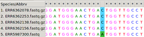
To do such calculation we need to first build an alignment of all the genomes (a multiple-sequence alignment, or MSA).
Afterwards, we will use specific software to analyze this MSA, count SNPs, and thus calculate the genetic distance between each pair of samples.
Figure 1: A SNP is highlighted in a MSA of five MTB genomes
Generate complete genomes
The first step to generate the genomes MSA will be… to get the complete genomes of our samples!
In the MTB Variant Analysis tutorial we have analyzed short-read high-throughput sequencing data (Illumina) to
obtain the respective VCF files that describe the mutations found in each of our samples, as compared
to the reference genome. We can now use these VCF files to build the complete genome of each of our
samples.
Filter VCF files for epidemiological/phylogenetic investigation
Interpreting mixed calls or indels in phylogenetic/epidemiological applications can be very
complicated. That is the reason why we typically use alignments that only contain fixed SNPs.
Thus, the first step in this tutorial will be to filter the VCFs so we are sure that
they only contain fixed SNPs, which we (somewhat arbitrarily) define as those single-nucleotide variants that are observed at an allele frequency of 90% or greater. We will be using the tool TB Variant Filter for this task.
Note: TB variant Filter refers to SNPs as SNVs. These two short forms are interchangeable, meaning Single Nucleotide Polymorphism and Single Nucleotide Variant, respectively.
Hands On: Filter VCF files for epidemiological investigation
TB Variant Filter ( Galaxy version 0.3.6+galaxy0) with the following parameters:
param-collection“VCF file to be filter”: MTB variants per sample; the uploaded collection of VCF datasets
“Filters to apply”: Only accept SNVs, Filter variants by percentage alt allele
“Show options for the filters”: Yes
“Minimum alternate allele percentage to accept”: 90.0
Question
TB Variant Filter reads the VCF and output only SNPs that have, at least, 90% frequency.
How can the software extract such information from the VCF datasets?
That information is contained, for each mutation, in the VCF:
The TYPE field within the INFO string will tell us if the mutation is a SNP (TYPE=snp)
You can look for other types of mutations like insertions (TYPE=ins)
The AF field within the INFO string describes the estimated Allele Frequency
In the absence of the AF field, the allele frequency can be calculated as: AO (alternate allele observations) / DP (depth of reads at the variant site)
Reconstruct the complete genome of each sample
Our new collection of VCF datasets now only contains fixed SNPs that were found in the genome of the respective strains.
Genomic positions not in the VCF mean that, at that particular position, the strain has the
same nucleotide than the reference genome. Knowing this information, one could reconstruct the
complete genome of each strain pretty easily. From the first to the last position in the genome,
one would put the same nucleotide than in the reference if that position is not in the VCF, or the
SNP described in the VCF otherwise. This is exactly what the tool bcftools consensus will do for us,
given the reference genome and the VCF of the strain we want to reconstruct the genome for.
Hands On: Reconstruct the complete genome of each sample
bcftools consensus ( Galaxy version 1.15.1+galaxy3) with the following parameters:
param-collection“VCF/BCF Data”: the collection of filtered variants per sample; output of TB Variant Filter
“Choose the source for the reference genome”: Use a genome from the history
param-file“Reference genome”: the uploaded MTB ancestor reference fasta dataset (the reference genome that was used for SNP-calling)
“Set output FASTA ID from name of VCF”: Yes
Question
Imagine that we forgot to filter the VCFs to contain only fixed variants, and there are also
SNPs with frequencies, of 15%, 30%, or 56.78%. Which allele do you think bcftools consensus would
insert in the genome?
The behaviour of bcftools consensus in this case can be specified with the option --haplotype
For example, we can set haplotype=2 so the second allele will be used… wait… what?
Question: Second allelle!?
What do you think that things like “second allele” or “The alterntive allele” mean here?
Many of the bioinformatic programs are developed to analyze eukaryotic genomes, particularly
human genomes. That means that these programs have in mind that the genomes
are diploid and thus each posible position in the genome has two possible alleles. In
bacterial genomics, in contrast, we are always sequencing a population of cells with
potential genetic diversity (with the exception of single-cell sequencing).
That does not mean that we cannot use this type of software, we can (and we do!) but it is
good to know what they are meant for, and their possible limitations.
Multiple-sequence alignment (MSA) of all genomes
Multiple sequence alignment is a process in which multiple DNA, RNA or protein sequences are arranged
to find regions of similarity that are supposed to reflect the consequences of different evolutionary
processes (Figure 1). MSAs are used to test hypotheses about these evolutionary processes and to infer phylogenetic
relationships, and for these reasons we build MSA for sequences for which we already assume some sort
of evolutionary relationship. You will learn more on MSAs and phylogenetic inference in the next
tutorial.
Building MSAs of several complete genomes can be a complicated process and computationally demanding. To perform
such a task there are many software packages available like Muscle, MAFFT or Clustal, just to mention some.
Which one are we going to use in this tutorial? Well, we are going to use a trick. We are going to
just stack one genome on top of each other within a text file. (More on why we can do this below).
Our aim is to generate a multifasta dataset in which the genomes of our samples are aligned.
Something that looks like this:
This could be done manually, by copy-pasting all genomes in a single text file.
However we can do the same with a specific command that concatenates datasets.
Hands On: Concatenate genomes to build a MSA
Concatenate datasets tail-to-head (cat) ( Galaxy version 0.1.1) with the following parameters:
param-collection“Datasets to concatenate”: the collection of consensus genomes; output of bcftools consensus
Now we have a multifasta file, where each position of each genome corresponds to the same position
of the rest of genomes in the file. This can be seen and used as a multiple-sequence alignment of
all of our genomes! However, it is important that you understand the following question…
Question
Generating multiple-sequence alignments can be complicated and computationally demanding, and there are
many software packages to perform such task. How is it possible that we were able to build a MSA by just
stacking genomes one on top of each other? Can you think about what makes our case special, so we can
just use this “trick”?
We have generated the complete genome of each sample by substituting in the reference genome
those SNPs that we found in that said sample (described in the VCF). Remember that we
removed indels from the VCF when filtering! Because the complete genomes we generated do not
contain insertions or deletions, ALL the genomes have the same length (the length of the
reference genome) and each nucleotide corresponds to the same genomic coordinate (the one
also in the reference genome). So we are not aligning genomes per se and, knowing this, we
can build a MSA by just stacking genomes that are the same length »AND« have the same coordinates.
Remove invariant positions
We have generated a MSA that is the basis for the transmission (clustering) and phylogenetic
analysis. Although we could already use this MSA for such analysis, it is common practice to remove
the invariant sites from the alignment. Think that our file now contains 20 genomes of 4.4 Mb each.
MTB genomes have a very low genetic diversity, meaning that in reality, there are only some hundreds or
thousands of SNPs in total, because the genomes are >99% identical between them. Identical positions
in a MSA provide no information, so we can remove those and
generate a SNP alignment that only contain variant positions with phylogenetic information. By
doing this, we will generate a much smaller file, that will be easier to handle by downstream applications.
We can exemplify this with a couple of pictures:
In the following picture, a polymorphic position in the alignment (SNP)
is highlighted in blue and green. Invariant positions are not highlighted and have an asterisc *
on the upper part of the alignment. Most of the MSA is composed of these invariant positions, making
our file larger than necessary.
Figure 3: A SNP alignment where all positions are polymorphic
Hands On: Removing invariant sites from a MSA
Finds SNP sites ( Galaxy version 2.5.1+galaxy0) with the following parameters:
param-file“FASTA file”: the concatenated consensus genomes; output of Concatenate datasets
“Output”: Sequence alignment / VCF
“Output formats”: Multi-FASTA alignment file
In SNP alignments you have to bear in mind that positions do not longer correspond to genomic
coordinates, meaning that two contiguous nucleotides may correspond to coordinates thousands of
positions apart.
Identify transmission clusters
Calculate pairwise SNP distances
Now we are all set to calculate pairwise SNP distances between samples and decide whether two
patients are within the same transmission cluster or not. Having a SNP alignment, this is fairly
easy. We will use SNP distance matrix, that will generate a matrix with pairwise SNP distances.
Hands On: Distance matrix from SNP alignment.
SNP distance matrix ( Galaxy version 0.8.2+galaxy0) with the following parameters:
param-file“FASTA multiple sequence alignment”: the concatenated SNP sites-only sequences; output of Finds SNP sites
Comment
Have a look at the distance matrix to make sure you understand the whole process. Given that
we only have 20 samples, you could already spot some samples that are involved in the same
transmission chain (samples with a small number of SNPs between them as explained below).
Determine transmission clusters based on a SNP threshold
Now that we have a distance matrix that describes the SNP distance between each pair of samples, we
could already describe the transmission clusters based on a SNP threshold, as explained in the
respective webinar . If two samples are at a distance below that threshold, we will say that they
belong to the same transmission cluster, because they are close enough genetically speaking. Again,
we could do this manually, but we are doing bioinformatics, and we want to be able to do the same
analysis regardless of whether we are analyzing two or two million samples. Also, note that two samples
that are dozens of SNPs apart may belong to the same transmission cluster if there are other samples
linking them in between as exemplified in the picture below.
Figure 4: Example of transmission cluster using 10 SNPs threshold
Question: Very Important Question
In the image above exemplifying a transmission cluster, the distance between samples A and E is
17 SNPs. Being the other pairwise distances in the figure the same,
would it be possible that the distance between A and E is different?
The figure used above as an example is a flagrant oversimplification. In the figure not all pairwise
distances are represented (for example between sample A and C).
Most importantly you have to remember that transmission clusters do not reflect transmission
events.
In fact it may happen that transmission does not happen within the cluster we are analyzing!
For example, when a patient that is not sampled is the source of infection of all the cases in
the cluster (may be a superspreading event). You have to consider that, taking into account the
same SNP distances, another possible (yet still oversimplified) scenario could be…
Figure 5: Example of transmission cluster using 10 SNPs threshold
Determine transmission clusters
The Galaxy team has implemented a tool that reads a SNP distance matrix like the one we just calculated and
assigns clusters based on a distance threshold. We will use this tool to perform a clustering with a threshold
of 12 SNPs.
Hands On: Distance matrix from SNP alignment.
Distance matrix-based hierarchical clustering tool metadata ( Galaxy version 1.1.1) with the following parameters:
param-file“Distance matrix”: SNP distance matrix; output of SNP distance matrix
“Generate cluster assignments?”: Yes, and use distance threshold to divide into clusters
“Distance threshold for sample clustering”: 12
Question
How many transmission clusters did we find? How many samples are linked to recent transmission in our dataset?
We have found two transmission clusters with respective IDs 1 and 2. Transmission cluster 1
is composed of two samples,ERR5987352 and ERR6362484 , linked by recent transmission and transmission cluster 2 of three samples, ERR6362138, ERR6362156 and ERR6362253.
Question
Let’s assume that we have the isolation dates of samples ERR6362484 and ERR5987352, which
belong to the same transmission cluster. Sample ERR6362484 was isolated on January 2021, while sample
ERR5987352 was isolated on September 2021. Would you be able to determine who was the infector and who the infectee?
NO
Isolation dates have been used traditionally to define index cases within transmission clusters
under the assumption that the most likely scenario is the first isolated sample to be the
source of transmission. Today we know that this assumption often leads
to misidentification of index cases. Remember: we cannot rule out the possibility
that patients within the cluster were infected by an index case that was not sampled.
Analysis Part 2: Combining cluster information with drug-resistance reports
Although we have stressed the fact that clustering cannot be used to delineate
transmission events, clustering is very useful to investigate outbreaks and determine which cases are
involved in the same transmission chain. We can leverage this information to investigate the relationship
between tuberculosis transmission and particular biological or clinical traits.
In this part of the tutorial, we will investigate the emergence and spread of drug resistance based
on our clustering analysis.
Get the data
The MTB Variant Analysis tutorial
demonstrates the use of TB-profiler to generate a report with determinants of drug resistance of a
particular MTB strain, and predict its genotypic drug susceptibility. We have done exactly the same
for the 20 samples that we used in the clustering analysis, so we have now the TB-profiler reports for
all of them.
Like in part 1, we can use Galaxy’s rule-based uploader functionality to upload the data, build a collection from it and name its elements correctly, all in one step.
In the bottom row of options, change Type from “Auto-detect” to txt
Set the name of the new collection to TB profiler reports
Click on Upload
Summarize the data
TB-profiler reports are very useful and comprehensive, and we will use them to better investigate
drug resistance in our dataset. However, it is always useful to summarize the data on a per-sample basis,
on a table, so we can quickly check which strains are, for example, MDR, an which are susceptible to antibiotics.
We would like to generate a table like the following:
Sample
DR profile
Sample A
Sensitive
Sample B
Sensitive
Sample C
MDR
Sample Z
XDR
and merge this with the tabular per-sample cluster report that we have generated in the first part of the tutorial.
If we take a look at a TB profiler report we can see that there is one line describing the genotypic drug susceptibility.
Let’s have a look at the first part of the TB-profiler report for sample ERR6362653:
TBProfiler report
=================

The following report has been generated by TBProfiler.

Summary
-------
ID: tbprofiler
Date: Fri Jan 28 13:14:47 2022
Strain: lineage2.2.1
Drug-resistance: MDR

Lineage report
--------------
Lineage	Estimated Fraction	Family	Spoligotype	Rd
lineage2	1.000	East-Asian	Beijing	RD105
lineage2.2	0.996	East-Asian (Beijing)	Beijing-RD207	RD105;RD207
lineage2.2.1	0.999	East-Asian (Beijing)	Beijing-RD181	RD105;RD207;RD181
As you can see, this strain is multi-drug resistant as indicated by (Drug-resistance: MDR)
We could then look for this information in each TB-profiler report and generate this table manually,
for example in a spreadsheet. However this is not feasible when analyzing hundreds or thousands of samples
(and very error-prone!).
A far more scalable approach is to combine Galaxy tools to automate the necessary data processing steps for us.
Select the line containing the drug resistance profile in the report of every sample
grep is used to search patterns of text within text files. Each time grep finds that
pattern, it will print as a result the complete line containing such pattern.
If we use grep to search for the pattern “Drug-resistance:”, in a TB-profiler file, we will get
as output the complete line, for example Drug-resistance: MDR
Hands On: Keep only `Drug-resistance:` lines from TB-profiler reports
Select lines that match an expression with the following parameters:
param-collection“Select lines from”: the uploaded collection of TB-profiler reports
“that”: Matching
“the pattern”: Drug-resistance:
Collapse collection into a table with each line prepended with a sample name
Next, we want to turn the collection of single-line datasets we just created into a single two-column table with
one column of sample IDs and another one with the corresponding drug resistance status.
Hands On: Prepend the sample name to the DR profile
Collapse Collection ( Galaxy version 5.1.0) with the following parameters:
param-collection“Collection of files to collapse into single dataset”: the collection of single-line drug-resistance reports; output of Select lines
“Prepend File name”: Yes
“Where to add dataset name”: Same line and each line in dataset
Clean up the table
In this step we will use a simple tool that searches and replaces text to remove the redundant string “Drug-resistance: “ from our table by replacing it with nothing.
Hands On: Removing redundant content
Replace Text ( Galaxy version 1.1.2) with the following parameters:
param-file“File to process”: Single file (output of Collapse Collectiontool)
In “Replacement”:
param-repeat“Insert Replacement”
“Find pattern”: Drug-resistance:
Note the space at the end of the pattern!
“Replace with”: leave this field empty
Once the tool has finished running, change the format of the output to tabular
Though by now the content of the dataset looks like a nice table, Galaxy still thinks it is in general txt format because the original TB-profiler reports were of that format.
Click on the galaxy-pencilpencil icon for the dataset to edit its attributes
In the central panel, click galaxy-chart-select-dataDatatypes tab on the top
In the galaxy-chart-select-dataAssign Datatype, select tabular from “New Type” dropdown
Tip: you can start typing the datatype into the field to filter the dropdown menu
Click the Save button
Question
How many MDR strains did we find in the dataset?
What does it mean to be Pre-MDR?
Eight MDR strains, three of which are pre-XDR because they have additional resistance to fluoroquinolones. (You can look into details by looking into the TB profiler reports).
As MDR means to be resistant to INH and RIF, pre-MDR means to be either INH-monoresistant or RIF-monoresistant.
If we have a look at the respective TB-profiler reports, we can see that these three strains are RIF-monoresistant.
Combine the drug-resistance and the cluster tables
The two tables we have generated in the two parts of the tutorial share a sample column, which we can use now to join the two tables.
Hands On: Joining tables
Join two files ( Galaxy version 1.1.2) with the following parameters:
param-file“2nd File”: final drug-resistance report; output of Replace Text above
“Column to use from 1st file”: Column: 1
“Output lines appearing in”: Both 1st & 2nd file
Interpretation of results
Now that we have performed a clustering analysis and know which DR mutations each strain carries,
we can try to answer a series of questions about how DR may have been emerging and spreading in our study
population.
The final combined table you generated and that we are going to base some questions on, should look similar to this one (header added and sample order rearranged for clarity here):
Sample
Cluster_id
DR profile
ERR1203059
-
Sensitive
ERR181435
-
Sensitive
ERR2659153
-
Sensitive
ERR2704678
-
Sensitive
ERR2704679
-
Sensitive
ERR2704687
-
Sensitive
ERR313115
-
Sensitive
ERR551620
-
MDR
ERR5987300
-
Pre-XDR
ERR6362078
-
MDR
ERR6362139
-
Pre-MDR
ERR6362333
-
Pre-XDR
ERR6362653
-
MDR
SRR13046689
-
Other
SRR998584
-
Sensitive
ERR5987352
1
Pre-MDR
ERR6362484
1
Pre-MDR
ERR6362138
2
MDR
ERR6362156
2
Pre-XDR
ERR6362253
2
MDR
Question
Assuming that we have a very good sampling of the outbreak. Which strains may represent instances
of de novo evolution of drug resistance and which ones instances of transmitted (primary) resistance?
Remember that you can look at the TB-profiler reports of independent samples for detailed information.
In a simplistic scenario, we could consider clustered strains as instances of transmission and
unclustered strains as instances of de novo evolution of DR. Thus, we see that for example there
are three MDR strains (ERR551620, ERR6362078, ERR6362653) that are unclustered and therefore may
represent cases in which drug resistance evolved independently as a consequence of treatment within the respective
patients. However you need to always bear in mind that, although within our population those MDR
strains do not seem to be linked to transmission, this does NOT rule out the possibility that
some of these patients were infected with an MDR strain somewhere else, or that other cases from the cluster where simply not sampled.
When looking at clustered strains, distinguishing between transmitted and de-novo may be tricky. Note
that, for example, for the two RIF-monoresistant strains linked within the same transmission
cluster there are, at least, a couple of possible scenarios: one in which a RIF-monoresistant strain
evolved in one patient and was transmitted to the other patient afterwards, and one in which both
were infected with the same RIF-monoresistant strain from a third patient that we have not sampled.
We need to note that, in the first scenario, drug resistance evolved de novo in one patient,
and was transmitted to the other patient, whereas in the second scenario drug resistance was
transmitted in both cases.
Question
The same principles as explained above apply to the three MDR strains that are
within the same transmission cluster. In this case, however, there is one strain that shows clear
evidence of de-novo evolution of DR. Do you know which strain and why?
Within this cluster of MDR strains, there is one tagged as Pre-XDR by TB-profiler. If we have
a look at the TB profiler report, we can see that this strain carries an additional mutation in
gyrA that confers resistance to fluoroquinolones. This is compatible with an scenario in which
fluoroquinolone resistance evolved independently within this patient after being infected with
the MDR strain.
Question
There is one strain with a DR profile “other”, because it is only resistant to pyrazinamide. This
strain is not within a transmission cluster. Therefore, we might conclude that pyrazinamide resistance
most likely evolved de-novo in this patient due to antibiotic treatment, but we would be wrong. Do you know why?
The strain is indeed PZA-resistant. And indeed this is strain is NOT linked to transmission
within our population. However, if we have a look at the TB-profiler report, we observe that this
is a M. bovis strain, many of which are known to be intrinsically resistant to PZA.
Question
Is it possible to find, in the same transmission cluster, two RIF-monoresistant strains that
carry different rpoB mutations?
Is it possible to find, in the same transmission cluster, strains of different MTB sublineages?
Yes, it is possible. In that scenario, the same susceptible strain would recently
have been transmitted to two patients, and RIF resistance would have evolved independently in both.
No, by definition. Remember that clustering is based on a threshold that we set of genetic
distance measured in SNPs. We want to cluster samples that are genetically so similar that we
can consider them as the same genotype, that is to say, as the same strain. Two different
sublineages, by definition, do not belong to the same genotype and will have a distance in SNPs
between them well beyond any SNP threshold we could use.
Conclusion
You have learned how to perform a clustering analysis to identify patients that are linked by events of
recent transmission. Clustering analysis is very useful in outbreak investigation and
can also be used to describe the emergence and spread of drug-resistance within a population. You have
also learned, however, that interpreting clustering results requires careful considerations, given the
limitations of the methodology. Clustering analysis is better complemented with phylogenetic analysis,
which may help overcome some of these limitations.
In the following tutorial you will perform a phylogenetic analysis of these same 20 strains.
Bonus
You might have noticed that one of the strains analyzed presents thousands of differences (SNPs) to
the reference genome, standing out from the rest of strains. This strain is a M. canettii strain,
that was actually not part of the outbreak investigated. However we decided to include it here. Why? Let’s find out
in the follow-up tutorial Tree thinking for tuberculosis evolution and epidemiology.
You've Finished the Tutorial
Please also consider filling out the Feedback Form as well!
Key points
Clustering is a useful tool to detect transmission links between patients and oubreak investigation.
Clustering can be used to investigate the transmission of certain traits, like drug resistance.
Clustering does not provide information about particular transmission events nor their directionality (who infected whom).
Clustering is very much influenced by sampling. Lower sampling proportions and shorter sampling timeframes lead to lower clustering rates that shoud not be confounded with lack of transmission.
Frequently Asked Questions
Have questions about this tutorial? Have a look at the available FAQ pages and support channels
Xu, Y., I. Cancino-Muñoz, M. Torres-Puente, L. M. Villamayor, R. Borrás et al., 2019 High-resolution mapping of tuberculosis transmission: Whole genome sequencing and phylogenetic modelling of a cohort from Valencia Region, Spain (M. B. Murray, Ed.). PLoS Med Medicine 16: e1002961. 10.1371/journal.pmed.1002961
Feedback
Did you use this material as an instructor? Feel free to give us feedback on how it went.
Did you use this material as a learner or student? Click the form below to leave feedback.
Hiltemann, Saskia, Rasche, Helena et al., 2023 Galaxy Training: A Powerful Framework for Teaching! PLOS Computational Biology 10.1371/journal.pcbi.1010752
Batut et al., 2018 Community-Driven Data Analysis Training for Biology Cell Systems 10.1016/j.cels.2018.05.012
@misc{evolution-mtb_transmission,
author = "Galo A. Goig and Daniela Brites and Christoph Stritt",
	title = "Identifying tuberculosis transmission links: from SNPs to transmission clusters (Galaxy Training Materials)",
	year = "",
	month = "",
	day = "",
	url = "\url{https://training.galaxyproject.org/training-material/topics/evolution/tutorials/mtb_transmission/tutorial.html}",
	note = "[Online; accessed TODAY]"
}
@article{Hiltemann_2023,
	doi = {10.1371/journal.pcbi.1010752},
	url = {https://doi.org/10.1371%2Fjournal.pcbi.1010752},
	year = 2023,
	month = {jan},
	publisher = {Public Library of Science ({PLoS})},
	volume = {19},
	number = {1},
	pages = {e1010752},
	author = {Saskia Hiltemann and Helena Rasche and Simon Gladman and Hans-Rudolf Hotz and Delphine Larivi{\`{e}}re and Daniel Blankenberg and Pratik D. Jagtap and Thomas Wollmann and Anthony Bretaudeau and Nadia Gou{\'{e}} and Timothy J. Griffin and Coline Royaux and Yvan Le Bras and Subina Mehta and Anna Syme and Frederik Coppens and Bert Droesbeke and Nicola Soranzo and Wendi Bacon and Fotis Psomopoulos and Crist{\'{o}}bal Gallardo-Alba and John Davis and Melanie Christine Föll and Matthias Fahrner and Maria A. Doyle and Beatriz Serrano-Solano and Anne Claire Fouilloux and Peter van Heusden and Wolfgang Maier and Dave Clements and Florian Heyl and Björn Grüning and B{\'{e}}r{\'{e}}nice Batut and},
	editor = {Francis Ouellette},
	title = {Galaxy Training: A powerful framework for teaching!},
	journal = {PLoS Comput Biol}
}
Congratulations on successfully completing this tutorial!
You can use Ephemeris's shed-tools install command to install the tools used in this tutorial.
4 stars:
Liked: Navigating through the platform, and finding solutions to some problem along
May 2026
5 stars:
Liked: The hand-on and explanations were easy to follow. I could visualize my output was quite exciting.
Disliked: I absolutely enjoyed the hands-on as I did not require assistance
5 stars:
Liked: The standard process
June 2024
5 stars:
Liked: Tools for identification of drug resistance and generating transmission cluster pattern
October 2023
4 stars:
Liked: Very clear tutorial
5 stars:
Liked: It was great to see that I achieved results by following the tutorial.
Disliked: In Part-1 Rstudio step was difficult to understand for me.
January 2023
4 stars:
Liked: All except the R studio that is not yet clear
Disliked: Rstudio
July 2022
4 stars:
Liked: This hands on tutorial made me understands some of the concepts raised in the webnar
Disliked: A note on the estimated run time of the on the provided data, this will help to know if i have done something wrong.
Questions:


 Open image in new tab
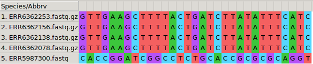 Open image in new tab
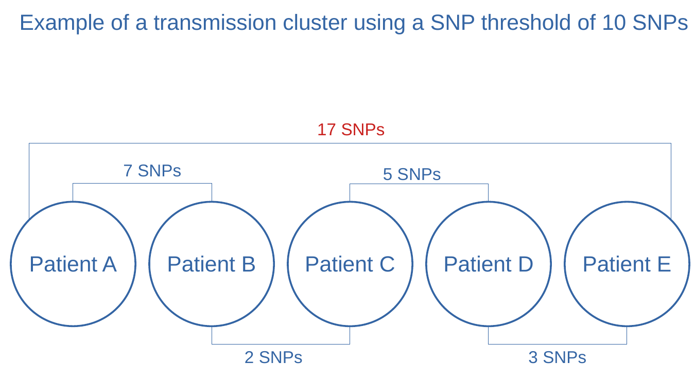 Open image in new tab
Open image in new tab
