Pox virus genome analysis from tiled-amplicon sequencing data
| Author(s) |
|
| Reviewers |
|
OverviewQuestions:
Objectives:
Which special challenges does one encounter during sequence data analysis of pox viruses?
How can standard workflows for viral mutation calling and consensus generation be adapted to the particularities of pox viruses?
How can viral consensus sequences, multiple-sequence alignments and mutation calls be generated from each other and used to answer questions about the data?
Requirements:
Learn how to deal with pox virus genomes inverted terminal repeats through a combination of wet lab protocol and tailored bioinformatics
Construct a sample consensus genome from mapped reads
Explore a recombinant pox virus genome via a multiple-sequence alignment of consensus genome and references and through lists of mutations derived from it
- Introduction to Galaxy Analyses
- slides Slides: Quality Control
- tutorial Hands-on: Quality Control
- slides Slides: Mapping
- tutorial Hands-on: Mapping
- tutorial Hands-on: Using dataset collections
- tutorial Hands-on: Rule Based Uploader
Time estimation: 4 hoursLevel: Advanced AdvancedSupporting Materials:Published: May 15, 2023Last modification: Mar 20, 2024License: Tutorial Content is licensed under Creative Commons Attribution 4.0 International License. The GTN Framework is licensed under MITpurl PURL: https://gxy.io/GTN:T00347rating Rating: 4.8 (0 recent ratings, 4 all time)version Revision: 4
Pox viruses (Poxviridae) are a large family of viruses, and members of it have various vertebrate and arthropod species as their natural hosts. The most widely known species in the family are the now extinct variola virus from the genus orthopoxvirus as the cause of smallpox, and vaccinia virus, a related, likely horsepox virus, which served as the source for the smallpox vaccine that allowed eradication of that disease.
However, various other pox viruses infect mammalian hosts and cause often severe diseases, and some of them have the ability to jump to humans. Mpox, caused by monkeypox virus, is the most recent and prominent example demonstrating the zoonotic potential of orthopoxviruses. The sister genus capripoxvirus is a major concern in livestock farming with all its three species - sheeppox virus (SPPV), goatpox virus (GTPV), and lumpy skin disease virus (LSDV) causing severe disease in sheep and goats (SPPV, GTPV) and in cattle (LSDV).
All pox viruses are characterized by a large double-stranded DNA genome (genome sizes of currently sequenced species range from 135 to 360kb) that gets replicated exclusively in the cytoplasm of host cells.
The ends of pox virus genomes consist of inverted terminal repeats (ITRs), i.e. regions of exact reverse-complementarity at the 5’- and 3’-end of the genome. At the very tips of the genome, these regions contain tandem repeats and terminal bases that are cross-linked to the opposite genome strand as first described for vaccinia virus and reviewed in Wittek 1982.
There is considerable length variation in the ITR regions of different species. For example, Capripox virus genomes have ITR lengths of 2.2 - 2.4 kb, monkeypox virus has 6.4 kb long ITRs, and variola virus had the shortest known ITRs with a length of just 700 bases (reviewed in Haller et al. 2014).
Independent of their size, ITRs pose a problem for the analysis of high-throughput sequencing data of pox viruses. Their repetitive nature can confuse de-novo assembly algorithms, but is, to some extent, also a challenge during reference-based mapping, particularly at the boundary between ITRs and the central region of the genome and with samples less related to the reference.
Recently, a tiled-amplicon approach with separate sequencing of half-genomes has been developed for capripoxviruses (Mathijs et al. 2022) that makes it possible to assign ITR-derived reads unambiguously to the 5’- or 3’-end of a pox virus genome when combined with a suitable bioinformatics pipeline.
This tutorial demonstrates how such data can be analyzed correctly with Galaxy.
Comment: Advanced tutorialThis tutorial demonstrates a very close to real-world analysis of viral sequencing data with Galaxy1. As such, it avoids many simplifications that are often made in training material to ease understanding. On the technical side, in particular, it makes use of many different Galaxy features and often assumes more than just basic familiarity with them. Like in other tutorials, you will find precise instructions for running every step in the analysis, but explanations focus very much on the biology of pox viruses and will often not offer much details on why a certain component of Galaxy is used the way it is described.
To get the most out of this tutorial, you should have worked through several other parts of the training material, which are listed under Requirements above, in particular:
- If you are not yet familiar with
- some typical ways of getting data into Galaxy,
- dataset collections and ways to manipulate them
- importing and running workflows,
you may benefit more from this tutorial if you first follow some of the introductory tutorials on these topics.
The tutorial also uses the rule-based uploader, which is an advanced feature, and treats it very much like a black box, which somehow lets you structure data exactly the way it is needed for the analysis. If you want to learn how to use this powerful feature for your own purposes, please follow the dedicated tutorials Rule Based Uploader and Rule Based Uploader Advanced.
- If this is your first exposure to sequencing data analysis, our more basic tutorials on quality control and mapping of such data are highly recommended to get you familiar with general concepts, data types, etc.
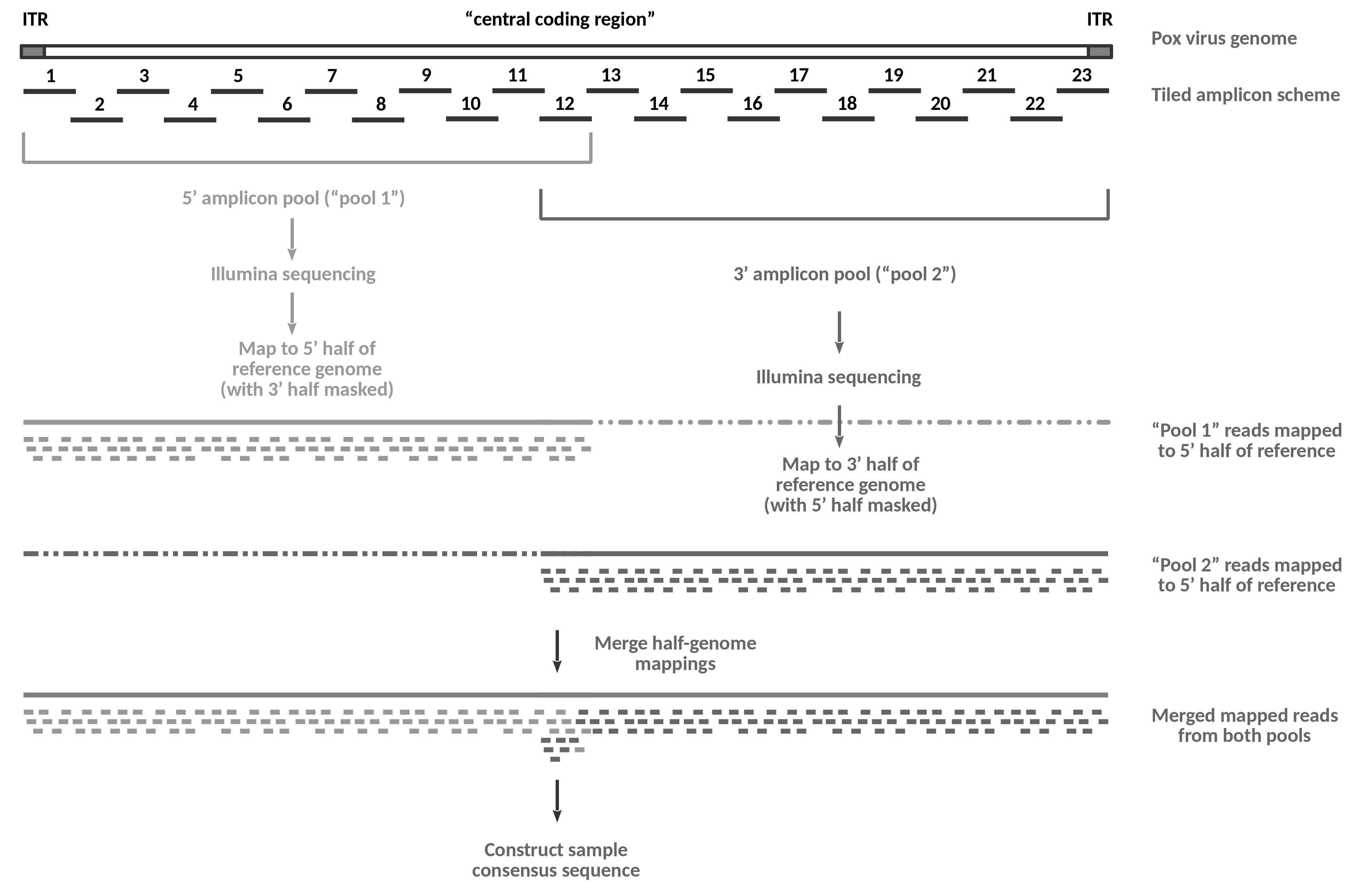
The following figure provides an overview of the wet lab data generation process described in Mathijs et al. 2022 and of the flow of the analysis that we will perform in this tutorial.
 Open image in new tab
On the wet lab side, the genome of a viral sample gets amplified in the form of 23 overlapping amplicons using a set of pan-genus primers suitable for all species of capripoxvirus.
Amplification happens in four separate multiplex PCR reactions: the primers for the odd-numbered amplicons (1-11) from the 5’ amplicon pool are used in reaction 1a, the primers for the even-numbered amplicons (2-12) in reaction 1b, the odd-numbered amplicons (13-23) from the 3’ amplicon pool in reaction 2a and the even numbered amplicons (12-22) from that pool in reaction 2b.
Note that the 5’-ITR gets amplified as part of amplicon 1, while the 3’-ITR is part of amplicon 23. Amplification of the two regions is specific because the right primer of amplicon 1 and the left primer of amplicon 23 both bind in the “central coding region”, i.e. outside the reverse-complementary ITRs.
After amplification, reactions 1a and 1b, and reactions 2a and 2b are combined to form the two sequencing pools, “pool 1” and “pool 2”. Note that amplicon 12 becomes part of both tools in the published protocol because overlap between the two sequencing pools is required for assembly-based analysis. For the mapping-based approach shown in this tutorial the overlap is not essential.
The DNA from the two pools is subjected separately to Illumina sequencing. This way, reads obtained from sequencing of “pool 1” are known to be derived from the 5’-half of the genome, while reads obtained from sequencing of “pool 2” are known to originate from the 3’-half.
In the tutorial analysis, we will exploit this information and map the “pool 1” data to a modified reference genome, in which the 3’-half of the sequence has been replaced with Ns. This masking prevents the read mapper from placing ambiguous reads (in particular reads derived from the 5’-ITR region) onto the 3’-half of the genome. Likewise, we will use a 5’-masked genome for the mapping of the “pool 2” reads, again preventing erroneous mapping of reads that we know must be derived from the 3’-half of the genome.
Once the correct alignments of the reads from the two pools have been recorded, we can safely merge the two results, and use that merged data to construct a consensus sequence for the sample.
Compared to a standard tiled-amplicon approach involving just one sequencing pool, the half-genome sequencing approach is more accurate, especially at the boundaries between the “central coding region” and the ITRs, but the analysis is complicated by the doubled number of inputs, by the need to generate masked reference sequences and by the extra step of merging two read mapping results.
AgendaIn this tutorial, we will cover:
- Prepare analysis history and data
- Generating masked reference genome versions for mapping
- Quality control of the sequencing data of all samples
- Mapping to the masked reference genomes
- Merging the mapped reads of both pools
- Mapped reads filtering, trimming, and QC
- Consensus sequence construction
- Quality check on results and interpretation
- Conclusion
- Footnotes
Prepare analysis history and data
Any analysis should get its own Galaxy history. So let’s start by creating a new one:
Hands On: Prepare the Galaxy history
Create a new history for this analysis
To create a new history simply click the new-history icon at the top of the history panel:
Rename the history
- Click on galaxy-pencil (Edit) next to the history name (which by default is “Unnamed history”)
- Type the new name:
pox-tiled-amplicon tutorial- Click on Save
- To cancel renaming, click the galaxy-undo “Cancel” button
If you do not have the galaxy-pencil (Edit) next to the history name (which can be the case if you are using an older version of Galaxy) do the following:
- Click on Unnamed history (or the current name of the history) (Click to rename history) at the top of your history panel
- Type the new name:
pox-tiled-amplicon tutorial- Press Enter

Get reference and sequenced samples data
In this tutorial you are going to work on the sequencing data from two samples of lumpy skin disease virus that have been sequenced as amplified half-genomes in Illumina paired-end mode. This means that we will be dealing with a forward and a reverse read dataset per sample and amplified half-genome, and so will have to download a total of eight sequenced reads datasets for our analysis.
The samples are the first two (SAMN20238786 and SAMN20238785) from BioProject PRJNA746718 as found through the European Nucleotide Archive browser.
If you follow the link, you should see that
-
for each of the two samples there is data from two sequencing runs (representing the two sequenced half-genome pools of amplicons).
If it isn’t shown by default, enable display of the Library Name column by clicking on Show Column Selection and selecting the checkbox for library_name. The pool identity (
1or2) is provided as the last part of each sequencing run’s library name. -
for each pool the data consists of two downloadable
fastq.gzresults files, which represent the forward and reverse reads for that sequencing run.
Comment: Choice of samplesAn in-depth analysis (Vandenbussche et al. 2022) of the samples from BioProject PRJNA746718 has revealed that their genomes are the result of recombination between at least two different parent strains. So not only are these samples sequenced following our wet lab protocol of choice, but there is also some prior knowledge about their (rather interesting) biology. This gives us the opportunity to evaluate the correctness of our analysis by comparing the results we will generate in this tutorial to the published findings.
In addition, we will require:
-
a reference genome to map the sequenced reads to
We will be using the public lumpy skin disease virus reference sequence NC_003027.1 from the NCBI RefSeq database here.
-
a primer scheme file with information about
- which amplicons were present in which half-genome sequencing pool
- where each primer binds with respect to the reference genome
This is a custom file, which you may have to modify, when analysing your own data, depending on the actual primer scheme used during sample preparation, and which we will just copy/paste into Galaxy. The version we are using describes the binding sites of the 46 primers published by (Mathijs et al. 2022) with respect to the NC_003027.1 reference sequence.
Hands On: Get the data
Import all pool 1 sequenced reads files of the two samples to analyze into your history.
You could collect the download links and additional metadata from the ENA page for
PRJNA746718, but for simplicity lets just use this precompiled combined information:20L81 ftp://ftp.sra.ebi.ac.uk/vol1/fastq/SRR151/074/SRR15145274/SRR15145274_1.fastq.gz 20L81 ftp://ftp.sra.ebi.ac.uk/vol1/fastq/SRR151/074/SRR15145274/SRR15145274_2.fastq.gz 20L70 ftp://ftp.sra.ebi.ac.uk/vol1/fastq/SRR151/076/SRR15145276/SRR15145276_1.fastq.gz 20L70 ftp://ftp.sra.ebi.ac.uk/vol1/fastq/SRR151/076/SRR15145276/SRR15145276_2.fastq.gzand upload them as a List of Pairs collection.
- Copy the links above
- Open the Upload Manager
- In the top row of tabs select Rule-based
- Set Upload data as to
Collection(s)- Paste the copied links into the text field on the right
- Click Build to bring up the Rule Builder dialog
- Click on the wrench icon tool next to Rules in the left panel of the window
In the text field, erase the prefilled content and copy/paste the following rule definition into it instead:
{ "rules": [ { "type": "add_column_regex", "target_column": 1, "expression": ".+_(\\d)\\.fastq\\.gz", "group_count": 1, "replacement": null } ], "mapping": [ { "type": "url", "columns": [1] }, { "type": "list_identifiers", "columns": [0], "editing": false }, { "type": "paired_identifier", "columns": [2] } ] }- Click on Apply
- In the bottom row of options, change Type from “Auto-detect” to
fastqsanger.gz- Set the name of the new collection to
pool1 reads- Click on Upload
It is ok to continue with the next step even while the upload of the pool 1 reads is still ongoing. Just click on the Close button of the information pop-up window if it is still open when you are ready to proceed.
Upload the pool2 sequenced reads files of the same samples using the corresponding metadata:
20L81    ftp://ftp.sra.ebi.ac.uk/vol1/fastq/SRR151/073/SRR15145273/SRR15145273_1.fastq.gz
20L81    ftp://ftp.sra.ebi.ac.uk/vol1/fastq/SRR151/073/SRR15145273/SRR15145273_2.fastq.gz
20L70    ftp://ftp.sra.ebi.ac.uk/vol1/fastq/SRR151/075/SRR15145275/SRR15145275_1.fastq.gz
20L70    ftp://ftp.sra.ebi.ac.uk/vol1/fastq/SRR151/075/SRR15145275/SRR15145275_2.fastq.gz
- Follow the same steps as for the pool 1 reads to get the data into your history.
- The rule definition used for the first pool will work unchanged for the second.
- Just make sure to choose
pool2 readsas the name of the new collection.As before, it is ok to proceed to the next step while the data upload is still ongoing.
Tag the uploaded collections of pool1 and pool2 reads
For each of the two collections
- Click on the collection in the history panel to step into it
- Click on the galaxy-pencil icon next to the collection name
- Click on “Add Tags”
- Use
#pool1and#pool2as the tag for the pool1 and the pool2 collection of reads, respectively- Click on galaxy-save Save
- Check that the tag appears below the collection name
Parts of the analysis in this tutorial will consist of identical steps performed on the data of each pool. To make it easier to distinguish which analysis step has been conducted with which pool, we will be using name tags. These are tags starting with
#, and they will automatically propagate to new datasets and collections derived from the tagged collections.Get the
NC_003027.1LSDV reference.A convenient public download link for this sequence is best obtained from the ENA again, where the sequence is known under its INSDC alias AF325528.1:
https://www.ebi.ac.uk/ena/browser/api/fasta/AF325528.1?download=true
Upload the reference to your history via the link above and make sure the dataset format is set to
fasta.
- Copy the link location
Click galaxy-upload Upload at the top of the activity panel
- Select galaxy-wf-edit Paste/Fetch Data
Paste the link(s) into the text field
Change Type (set all): from “Auto-detect” to
fastaPress Start
- Close the window
- Replace Text in entire line ( Galaxy version 1.1.2) to simplify the reference sequence name
- param-file “File to process”: the uploaded reference sequence from the ENA
- In param-repeat “1. Replacement”:
- “Find pattern”:
^>.+- “Replace with”:
>AF325528.1When the Replace Text tool run is finished, rename the output dataset
- Click on the galaxy-pencil pencil icon for the dataset to edit its attributes
- In the central panel, change the Name field to
LSDV reference- Click the Save button
Upload the primer scheme information in BED format
NC_003027.1    235       264       CaPV-V1_1_LEFT      pool1a    +
NC_003027.1    6789      6819      CaPV-V1_2_LEFT      pool1b    +
NC_003027.1    7771      7801      CaPV-V1_1_RIGHT     pool1a    -
NC_003027.1    13515     13543     CaPV-V1_3_LEFT      pool1a    +
NC_003027.1    14451     14482     CaPV-V1_2_RIGHT     pool1b    -
NC_003027.1    20192     20219     CaPV-V1_4_LEFT      pool1b    +
NC_003027.1    21201     21229     CaPV-V1_3_RIGHT     pool1a    -
NC_003027.1    26787     26814     CaPV-V1_5_LEFT      pool1a    +
NC_003027.1    27786     27814     CaPV-V1_4_RIGHT     pool1b    -
NC_003027.1    33277     33305     CaPV-V1_6_LEFT      pool1b    +
NC_003027.1    34363     34395     CaPV-V1_5_RIGHT     pool1a    -
NC_003027.1    39894     39921     CaPV-V1_7_LEFT      pool1a    +
NC_003027.1    40867     40897     CaPV-V1_6_RIGHT     pool1b    -
NC_003027.1    46393     46420     CaPV-V1_8_LEFT      pool1b    +
NC_003027.1    47419     47453     CaPV-V1_7_RIGHT     pool1a    -
NC_003027.1    52864     52890     CaPV-V1_9_LEFT      pool1a    +
NC_003027.1    54039     54069     CaPV-V1_8_RIGHT     pool1b    -
NC_003027.1    59439     59472     CaPV-V1_10_LEFT     pool1b    +
NC_003027.1    60530     60559     CaPV-V1_9_RIGHT     pool1a    -
NC_003027.1    66008     66041     CaPV-V1_11_LEFT     pool1a    +
NC_003027.1    66960     66989     CaPV-V1_10_RIGHT    pool1b    -
NC_003027.1    72534     72560     CaPV-V1_12_LEFT     pool1b    +
NC_003027.1    72534     72560     CaPV-V1_12_LEFT     pool2b    +
NC_003027.1    73568     73601     CaPV-V1_11_RIGHT    pool1a    -
NC_003027.1    79081     79111     CaPV-V1_13_LEFT     pool2a    +
NC_003027.1    80176     80202     CaPV-V1_12_RIGHT    pool1b    -
NC_003027.1    80176     80202     CaPV-V1_12_RIGHT    pool2b    -
NC_003027.1    85743     85777     CaPV-V1_14_LEFT     pool2b    +
NC_003027.1    86753     86781     CaPV-V1_13_RIGHT    pool2a    -
NC_003027.1    92208     92232     CaPV-V1_15_LEFT     pool2a    +
NC_003027.1    93323     93351     CaPV-V1_14_RIGHT    pool2b    -
NC_003027.1    98974     99002     CaPV-V1_16_LEFT     pool2b    +
NC_003027.1    99970     100000    CaPV-V1_15_RIGHT    pool2a    -
NC_003027.1    105634    105662    CaPV-V1_17_LEFT     pool2a    +
NC_003027.1    106584    106612    CaPV-V1_16_RIGHT    pool2b    -
NC_003027.1    112082    112108    CaPV-V1_18_LEFT     pool2b    +
NC_003027.1    113111    113144    CaPV-V1_17_RIGHT    pool2a    -
NC_003027.1    118617    118649    CaPV-V1a_19_LEFT    pool2a    +
NC_003027.1    119649    119675    CaPV-V1_18_RIGHT    pool2b    -
NC_003027.1    125361    125390    CaPV-V1_20_LEFT     pool2b    +
NC_003027.1    126297    126328    CaPV-V1_19_RIGHT    pool2a    -
NC_003027.1    131713    131742    CaPV-V1_21_LEFT     pool2a    +
NC_003027.1    132961    132988    CaPV-V1_20_RIGHT    pool2b    -
NC_003027.1    138437    138467    CaPV-V1_22_LEFT     pool2b    +
NC_003027.1    139333    139365    CaPV-V1_21_RIGHT    pool2a    -
NC_003027.1    143117    143145    CaPV-V1_23_LEFT     pool2a    +
NC_003027.1    146188    146219    CaPV-V1_22_RIGHT    pool2b    -
NC_003027.1    150505    150538    CaPV-V1_23_RIGHT    pool2a    -
Since BED is a tabular format, but the above display uses spaces to separate columns, please make sure, you have Convert spaces to tabs checked when creating the dataset from the copied content!
- Click galaxy-upload Upload Data at the top of the tool panel
- Select galaxy-wf-edit Paste/Fetch Data at the bottom
Paste the file contents into the text field
- Change the dataset name from “New File” to
LSDV primer scheme- Change Type from “Auto-detect” to
bed* From the Settings menu (galaxy-gear) select Convert spaces to tabs* Press Start and Close the window

At this point you should have these four items in your history:
- The collection of pool 1 reads (representing the 5’-half of the genome)
- This should be a list of two elements (representing the two samples we are going to analyze).
- Each of these elements should itself be a paired collection of a forward and a reverse reads dataset in
fastqsanger.gzformat. - A
#pool1name tag should be attached to the collection in the history.
- The collection of pool 2 reads (representing the 3’-half of the genome)
- This should be structured exactly as the first collection.
- Also the names of the elements in both collections should be identical.
- A
#pool2name tag should be attached to the collection in the history.
- The LSDV reference as a single fasta dataset
- The primer scheme as a single bed dataset
If this is the case for you, you are ready to start the actual data analysis.
Generating masked reference genome versions for mapping
As illustrated in Figure 1, we would like to map the “pool 1” reads of each sample to a version of the LSDV reference, in which the 3’-half of the genome (starting after the right end of amplicon 12, the 3’-most amplicon still contained in pool 1) is masked (i.e., bases are replaced by Ns). This ensures that the read mapper will only consider the 5’-half of the genome when placing reads from pool 1. Likewise, for the “pool2” read mapping, we would like to use a reference version, in which the 5’-half that is not covered by the second amplicon pool is masked out.
To build these two masked reference versions we need to extract the information about amplicon pool boundaries from the primer scheme BED dataset and use it twice on the LSDV reference to replace the appropriate ranges of its bases with Ns.
As this is a complex task that would take a considerable amount of time to perform step-by-step via manual tool runs, we are providing a pre-built workflow for you that you only need to import and run on the input data in your history.
Hands On: Import and run the reference masking workflow
- Go to the training material page for this workflow and use one of the options listed there to import the workflow into your account on your Galaxy server.
- Back on the list of workflows page, click the Run workflow icon workflow-run to the right of the newly imported workflow.
- On the next page, select
- “Primer Scheme (BED file with Pool identifiers)”: the uploaded
LSDV primer schemeBED dataset- “Reference FASTA”: the
LSDV referencefasta dataset generated with Replace TextRunning the workflow will produce two key output datasets:
- a Masked reference for mapping of pool1
- a Masked reference for mapping of pool2
Check whether the workflow produced correctly masked half-genomes
You can galaxy-eye inspect the two masked reference datasets by eye, which quickly reveals that one sequence has its beginning N-masked, while for the other it is the end, but it is hard to find out whether the regions are exactly right this way. Luckily, we can use a tool to determine the exact extent of Ns for each dataset:
- Fasta regular expression finder ( Galaxy version 0.1.0)
- param-files “Input”: select the two masked reference datasets; output of the masking workflow run
“Regular expression”:
N+This looks for stretches of one or more Ns.
- In “Specify advanced parameters”:
“Do not search the reverse complement”:
YesWe are only interested in the forward strand (and an N is an N on both strands anyway) so we can save some compute by turning on this option.
“Maximum length of the match to report”:
1It would be boring to have the matched stretches of Ns written out again.
QuestionInspect the two result datasets created by the tool and compare the regions of Ns reported in them to the primer scheme. Did the correct regions get masked?
Tip: Galaxy’s galaxy-scratchbook Window Manager, which you can enable (and disable again) from the menu bar can be very helpful for comparing multiple datasets.
The masked reference for mapping of pool1 has Ns from 80,202 - 150,773. The 3’-most primer contained in pool1, CaPV-V1_12_RIGHT, has its binding site listed as 80,176 - 80,202. Bed format specifies zero-based half-open intervals, i.e. the first base of a sequence has position 0, and the end position of any interval is the first base not included in it! So the 3’-most base covered by the primer is base number 80,201 (when counting from 0) and the reference is masked correctly from 80,202 onwards.
The masked reference for mapping of pool2 has Ns from 0 - 72,534. The 5’-most primer of pool2 is CaPV-V1_12_LEFT and the primer scheme lists the start of its binding site as 72,534. Again, the way bed format is specified means that position 72,534 is the first base not masked in the reference for pool2 mapping, and that is correct. Also note that amplicon 12 is contained in both pools and the masking takes this fact into account.
Feel free to open the workflow in the workflow editor and inspect the steps it took to work out the masking, but it’s also ok to treat this part as a black box and move on. There is still a lot of analysis that is waiting to be done.
Quality control of the sequencing data of all samples
The next step is to check the quality of the sequencing data of both samples and to eliminate, if necessary, poor-quality reads or parts of them.
The tool fastp lets us perform these tasks and obtain a nice quality report for our reads before and after processing in one go, but many other options exist to perform sequenced reads quality control and trimming/filtering in Galaxy, and the dedicated tutorial on quality control introduces more of them.
Hands On: QC and read trimming/filtering with fastp
- fastp ( Galaxy version 0.23.2+galaxy0) on the collection of pool1 reads
- “Single-end or paired reads”:
Paired Collection- “Select paired collection(s)”: the uploaded collection of pool1 reads
- In “Filter Options”
- In “Length filtering options”
- “Length required”:
30fastp comes with basic default settings for some of its many parameters. In particular, with no explicit parameter specifications, the tool will still remove reads that
- have base qualities < 15 for more than 40% of their bases
- have more than 5 Ns in their sequence
have a length < 15 bases (after removing poly-G tails from Illumina reads)
Because our input data has far longer MiSeq-generated reads, we can increase this length threshold to 30 bases as done above.
These are very relaxed criteria that will only remove the least usable reads, but still assure minimal quality standards that are good enough for many (including training) purposes.
Running the tool will result in two outputs. One is a new paired collection with the processed reads, the other one is a report of initial quality, the processing actions performed and their effect on key quality metrics.
galaxy-eye Inspect the reports for both samples and try to answer the following questions:
Question: Questions
- After filtering, which of the two samples has more reads retained?
- Which sample had more reads filtered out?
- Sample 20L81 has more reads retained (947,000) than 20L70 (856,000).
- Sample 20L81 also had more reads filtered out. “Only” 93.2% of its original reads got retained compared to 99.1% for 20L70.
Now repeat the steps above for the collection of pool 2 reads.
fastp ( Galaxy version 0.23.2+galaxy0) on the collection of pool2 reads
- “Single-end or paired reads”:
Paired Collection- “Select paired collection(s)”: the uploaded collection of pool2 reads
- In “Filter Options”
- In “Length filtering options”
- “Length required”:
30Question: Questions
- Are the results for the pool 2 sequences similar to those of pool 1?
- What’s your overall conclusion regarding the quality of the sequences and the effect of filtering?
- Results are rather similar although for pool2 the metrics for the two samples are even more similar than for poo1, and it is now 20L70, which has a bit more reads retained after filtering.
- The input sequences are of rather good quality and the relaxed filtering criteria we have configured had little impact. This is not a bad thing though and we can proceed with our analysis.
Mapping to the masked reference genomes
We are now ready to map each pool of each sample to the corresponding masked reference. We will use the tool BWA-MEM with essentially default settings for this purpose. As shown in figure 1, however, we want to merge the mapping results afterwards, but still be able to tell mapped reads from pool 1 and pool 2 apart. To this end, we need to tag reads with pool1 and pool2 read group identifiers, respectively, at the mapping step. Just because a sample has pool1 and pool2 reads it is still just one sample though, and we are going to express that fact through a common sample name (which we let BWA-MEM autodetect as the name of the collection elements).
Hands On: Read mapping and quality control
- Map with BWA-MEM ( Galaxy version 0.7.17.2) for pool1 data
- “Will you select a reference genome from your history or use a built-in index?”:
Use a genome from history and build index
- param-file “Use the following dataset as the reference sequence”: Masked reference for mapping of pool1
- “Single or Paired-end reads”:
Paired Collection- “Select a paired collection”: the
#pool1collection of trimmed and filtered reads; output of fastp run on the pool1 data“Set read groups information?”:
Set read groups (SAM/BAM specification)for Read group identifier:
- “Auto-assign”:
No- “Read group identifier”:
pool1for Read group sample name:
“Auto-assign”:
YesThis interprets names of collection elements as sample names.
- Map with BWA-MEM ( Galaxy version 0.7.17.2) for pool2 data
- “Will you select a reference genome from your history or use a built-in index?”:
Use a genome from history and build index
- param-file “Use the following dataset as the reference sequence”: Masked reference for mapping of pool2
- “Single or Paired-end reads”:
Paired Collection- “Select a paired collection”: the
#pool2collection of trimmed and filtered reads; output of fastp run on the pool2 data“Set read groups information?”:
Set read groups (SAM/BAM specification)for Read group identifier:
- “Auto-assign”:
No- “Read group identifier”:
pool2for Read group sample name:
- “Auto-assign”:
Yes
Merging the mapped reads of both pools
We have mapped both pool 1 and pool 2 reads to masked versions of the same reference sequence. This means that any mapping in any of the separate BWA-MEM outputs also describes a valid mapping to the complete, unmasked reference so all we need to do is merge the pool 1 and pool 2 mapped reads datasets of each sample into one to obtain complete mapping results for the entire genome of the sample.
A tool that can perform this task for us is samtools merge. However, if we gave this tool our collection of pool1 reads with one BAM dataset per sample and the collection of pool2 reads with again one BAM dataset per sample, you would be very disappointed to see that it would merge all datasets into one, i.e. it would not only combine pools, but also sample data, which is not what we want.
Why does samtools merge in Galaxy behave like this? Well, the tool is written so that it knows how to merge multiple datasets and it knows how to merge the contents of simple collections - and it’s just too eager to apply that knowledge. What we can do, however, is try and pass it something it does not know how to handle in a single run, and that’s a nested collection. So instead of providing the input as two separate collections (one for pool1 and one for pool2 data) that each hold two elements (representing data from one sample), we want to provide a collection of two samples, each one consisting of a collection of pool 1 and pool 2 reads, in turn. When we do this, Galaxy will recognize that the tool cannot handle this, but that it would know how to handle each outer element (sample) separately (as a simple collection). In this situation, Galaxy will automatically schedule two parallel excutions of the tool for us, each one receiving one element of the outer collection as input.
We can do the necessary restructuring in two steps, then pass the result to samtools merge.
Hands On: Reorganize the data and merge across pools within samples
- Zip collections with the following parameters
- param-collection “Input 1”: mapped reads
#pool1; output of BWA-MEM run on the pool1 data- param-collection “Input 2”: mapped reads
#pool2; output of BWA-MEM run on the pool2 dataThis combines the two separate collections into one nested structure, but, unfortunately, that structure is not organized the way we want it because Zip collections creates lists of pairs, i.e. list collections that hold paired collections inside. Now we still need to turn the list of pairs into a list of lists.
- Apply rules with the following parameters
- “Input Collection”: zipped collection of mapped reads from both pools
- Under “Rules”
- galaxy-wf-edit Edit
- In the “Build Rules for Applying to Existing Collection” window
- Click tool next to Rules
- Erase the prefilled rules description
Copy the rules below and paste them into the empty rules description area
{ "rules": [ { "type": "add_column_metadata", "value": "identifier0" }, { "type": "add_column_metadata", "value": "identifier1" } ], "mapping": [ { "type": "list_identifiers", "columns": [ 0, 1 ], "editing": false } ] }- Click Apply
- Click Save, then run the tool
This will reorganize the data once more, this time into the desired structure, which will give us the correct merge result.
- Samtools merge ( Galaxy version 1.15.1+galaxy0)
- param-collection “Alignments in BAM format”: the reorganized collection; output of Apply rules
- “Make @RG headers unique”:
No- “Make @PG headers unique”:
Yesgalaxy-eye Now lets confirm that things have worked as expected:
Question: Questions
- What are the datasets inside the Samtools merge collection?
- galaxy-eye Display each of the datasets. What information about read groups and samples is stored in each dataset?
- The collection consists of two BAM datasets, one for sample 20L81 and one for 20L70.
The header of the 20L81 dataset lists
@RG ID:pool1 SM:20L81 PL:ILLUMINA
@RG ID:pool2 SM:20L81 PL:ILLUMINA
, which declares that the mapped reads in this file come from two read groups with the IDs pool1 and pool2 that belong to the same sample (SM), 20L81, sequenced on the Illumina platform.
The 20L70 dataset contains analogous lines in its header declaring the two read groups of the other sample.
When scrolling to the very right in the body of the datasets, you can see that a RG tag of the form RG:ID (where ID is one of the alternatives declared in the header) is attached to each mapped read line (because the dataset is sorted by mapped coordinates and pool2 reads should have been mapped only to the 3’-half of the genome, you will have to scroll down rather far in the dataset to find a RG tag with a pool2 ID value).
All this read group information in the dataset headers and on the mapped reads has been put there by BWA-MEM and Samtools merge has, apparently, merged the reads and the read group information correctly!
Mapped reads filtering, trimming, and QC
So now that we have one dataset of mapped reads per sample, we will do some cleaning and quality control on the mapped data to be sure we pass only reliable mapping data into consensus calling.
We will first use samtools view to discard any alignments that we are not fully confident in.
Next, we will run ivar trim on the retained reads. This tool can detect primer sequences at the ends of the mapped reads that represent the tiled amplicon primers used during preparation of the samples for sequencing, and will mask them so that they will not be considered during generation of the consensus sequence.
The primers used for the tiled-amplicon generation will get incorporated physically at the start and end of each amplicon. These ends, therefor, do not represent amplified sequence from the sample genome, but merely reflect the primer sequences. Consequently, the amplicon ends will never capture any mutations in the genome region they cover, and we cannot meaningfully use them for building a consensus sequence for the sample.
Luckily, since we are dealing with tiled (i.e., overlapping) amplicons, each amplicon end should be overlapped by the non-primer part of another amplicon, and we can use these sequences to obtain information about the sequenced sample at primer binding sites. By masking parts of reads that are derived from incorporated primers, we make sure these “pseudo”-sequences are not interfering with mutation detection based on truly informative reads, and that we can faithfully reconstruct the genome of the sample.
Finally, we will use Qualimap BamQC to generate a quality report on the trimmed and filtered mapped reads, which we’ll inspect to judge whether read mapping worked well enough for consensus generation purposes.
Hands On: Mapped reads filtering and trimming and quality control for mappings
- Samtools view ( Galaxy version 1.15.1+galaxy0) for filtering the mapped reads
- param-collection “SAM/BAM/CRAM data set”: collection of merged mapped reads; output of Samtools merge
- “What would you like to look at?”:
A filtered/subsampled selection of reads- In “Configure filters”:
- “Filter by quality”:
20- “Require that these flags are set”:
Read is paired- “Exclude reads with any of the following flags set”:
Read is unmappedandMate is unmappedandAlignment of the read is not primaryandAlignment is supplementary- ivar trim ( Galaxy version 1.4.2+galaxy0) for trimming of amplicon primers from mapped reads
- param-collection “BAM file”: collection of filtered mapped reads BAM dataset; output of Samtools view
- “Source of primer information”:
History
- “BED file with primer sequences and positions”: the uploaded
LSDV primer schemeBED dataset- “Filter reads based on amplicon info”:
Yes, drop reads that extend beyond amplicon boundaries- “Include reads not ending in any primer binding sites?”:
Yes- “Require a minimum length for reads to retain them after any trimming?”:
Yes, and provide a custom threshold
- “Minimum trimmed length threshold”: `30
- QualiMap BamQC ( Galaxy version 2.2.2d+galaxy3) for mapped reads quality control
- param-collection “Mapped reads input dataset”: filtered and trimmed mapped reads BAM dataset; output of ivar trim
- “Skip duplicate reads”:
Deselect all- In “Settings affecting specific plots”:
- “Number of bins to use in across-reference plots”:
200galaxy-eye Study the report generated with QualiMap
Question: Questions
- What is the mean coverage for each of the samples across the entire genome?
- Which sample might be a bit more problematic coverage-wise?
- What can you observe for the “Mapping Quality Across Reference” plots for both samples?
- Mean coverage for sample 20L81 is 2,073, for 20L70 it is 2,155.
Despite its slightly higher mean coverage, sample 20L70 has the slightly worse coverage distribution.
The “Coverage across reference” plot shows higher variability of coverage for this sample. While it peaks at higher values, it also drops below a coverage of 500 more clearly and in more regions across the genome than 20L81, and even drops to potentially problematically low values in a short stretch of sequence just after the middle of the genome. The “Coverage Histogram” plot also reveals that the coverage distribution for 20L70 is a bit skewed towards lower values than that for 20L81.
All these effects are not very dramatic and should not prevent us from continuing with the analysis of both samples. We should watch out for a potentially incomplete consensus sequence in that low-coverage stretch of the 20L70 genome though.
- Mapping quality is almost constant at or very near 60 (which happens to be the maximum mapping quality value emitted by BWA-MEM) across the entire genome for both samples. Interestingly, there is a tiny dip in mapping quality around ~ 117,000 - 118,000 on the genome, which seems reproducible across the two samples.
Consensus sequence construction
And with that we are ready for consensus sequence generation!
To accept any base suggested by the mapped sequenced reads as the consensus base for the corresponding genome position, we ask for the following requirements to be fulfilled:
- at least 20 sequenced reads have to provide information about the base in question
- at a minimum, 70% of these reads have to agree on the base at this position (80% for indels)
To avoid getting misled too much by sequencing errors, we are also going to ignore bases with a base calling quality less than 20 in the above counts (i.e., we are going to base our decisions only on bases in sequenced reads that the basecaller of the sequencer was reasonably sure about.
Now what if we cannot obtain a consensus base for a position with the above criteria? In such cases of uncertainty we want to insert an N (i.e. an unknown base) to express that we either did not have enough information about the position or that this information was ambiguous.
galaxy-info All of the above limits for consensus base calling are arbitrary to some degree, and depend somewhat on the quality of the sequencing data. With very high overall coverage, for example, it is possible to increase the coverage threshold, but if you increase that threshold too much, you may end up with a consensus sequence consisting mostly of Ns.
Hands On: Consensus building
- ivar consensus ( Galaxy version 1.4.2+galaxy0)
- param-collection “BAM file”: collection of trimmed mapped reads BAM dataset; output of ivar trim
- “Minimum frequency threshold”:
0.7- “Minimum indel frequency threshold”:
0.8- “Minimum depth to call consensus”:
20galaxy-eye Inspect the consensus sequences generated for the two samples
QuestionDoes everything look ok? What about those leading and trailing Ns in the sequences?
Certainly both sequences start and end with stretches of Ns.
Since the sequencing data is ampliconic in nature, and the primer scheme lists the first and the last primer as binding close to but not exactly at the end of the genome, it is expected that we cannot resolve the first and last couple of hundreds bases.
However, to determine whether those terminal stretches of Ns are exactly as long as we expect them to be would be a tedious task to perform manually. Likewise, it is not trivial to assert that there are no additional Ns somewhere in these long sequences.
Quality check on results and interpretation
Composition of the consensus sequences
So we have consensus sequences for our samples. Are there better ways for checking their quality than just looking through them by eye?
Luckily, there is a tool to help us, and we have even used it before to check the masking of the reference genome!
Hands On: Check consensus sequences for unresolved bases
- Fasta regular expression finder ( Galaxy version 0.1.0)
- param-collection “BAM file”: collection of consensus sequences; output of ivar consensus
“Regular expression”:
[^ATGC]+This expression matches stretches of sequences that do not (
^) contain any of the standard bases (any of the characters in[]). The expression is case-sensitive, but ivar consensus only uses uppercase in sequences.- In “Specify advanced parameters”:
- “Do not search the reverse complement”:
Yes- “Maximum length of the match to report”:
1galaxy-eye Inspect the output of the tool for both samples and compare it to the primer scheme
QuestionHas consensus building worked well?
The tool reports only two stretches consisting of Ns at both ends of the genome, and their positions are exactly identical between the samples. There are no interior Ns, nor other ambiguity characters.
The 5’-end stretch of Ns extends up to position 264 (in bed format, so zero-based and the position itself not included). The binding site of the first primer in the primer scheme is from (bed format again) 235 up to 264.
Remember that we used ivar trim to mask primer sequences? This seems to have worked well, and we got a consensus sequence from the first position for which we could reasonably expect information!
The 3’-end stretch of Ns starts at position 150,453 and continues (as we have seen by eye before) until the end of the genome, which seems to be at 150,721. Hmm, these values are surrounding the binding site of the last primer in the primer scheme, but do not match perfectly. But wait:
It is possible that the consensus sequences incorporate deletions, i.e. it could be that they are shorter than the reference we have used for mapping. So obviously the consensus sequences have a length of 150,721 bases, but what is the length of the reference?
There are Galaxy tools for determining the length of a FASTA sequence. For example, you could use Compute sequence length ( Galaxy version 1.0.3) on the
LSDV referencedataset, but we have obtained the value before when we used the Fasta regular expression finder on the reference masked for pool 1 mapping. So lets try to find that output in the history and see what it says:Chrom Start End Name Score Strand ThickStart AF325528.1 80201 150773 AF325528.1_80201_150773_for 70572 + N[1,70572]is what the tool reported for the 3’-mask so the reference is 150,773 bases long.
Now, 150,773 - 150,721 = 52 is how many bases the consensus sequences are shorter than the reference, and on these shorter sequences the binding site of the 3’-most primer would be shifted from 150,505 - 150,538 on the reference to 150,453 - 150, 486.
Again primer masking by ivar trim will cause the primer sequence itself to be ignored during consensus sequence building so we can expect the sequence to be resolved up to position 150,453 and this is exactly where the trailing Ns start.
Consensus building seems to have worked perfectly, with no interior Ns and the maximal sequence resolved!
Confirmation of published findings
Even a perfectly looking consensus sequence could, of course, have wrong bases incorporated. Also, a consensus sequence on its own does not convey too much information.
So the next question is if the sequences we have generated make sense when compared to other sequences.
Figure 2 in (Vandenbussche et al. 2022) illustrates that our two samples (third-last and fourth-last alignment records in both panels A and B) have a mosaic genome composed of recombined sequences from at least two different parent strains, and as a plausibility check we can try to reproduce this finding.
For this, we will need to create a multiple-sequence alignment (MSA) between our consensus sequences and the assumed parent strains used in the figure. The assumed parent P2 (with accesion number KX683219), however, is very closely related to the reference we have used for mapping here so we can simply use that already obtained sequence instead of parent P2.
This leaves us with the tasks of obtaining the sequence for parent P1 (accession number: KX764644) and of combining this sequence, our reference and our two consensus sequences into an MSA.
Hands On: Build multiple-sequence alignment between samples and two LSDV references
Get the
KX764644LSDV “Herbivac” reference.As with the LSDV reference sequence that we have used for mapping, we can use a convenient download link for the Herbivac strain sequence at the ENA:
https://www.ebi.ac.uk/ena/browser/api/fasta/KX764644.1?download=true
Upload the reference to your history via the link above and make sure the dataset format is set to
fasta.
- Copy the link location
Click galaxy-upload Upload at the top of the activity panel
- Select galaxy-wf-edit Paste/Fetch Data
Paste the link(s) into the text field
Change Type (set all): from “Auto-detect” to
fastaPress Start
- Close the window
- Replace Text in entire line ( Galaxy version 1.1.2) to simplify the reference sequence name
- param-file “File to process”: the uploaded reference sequence from the ENA
- In param-repeat “1. Replacement”:
- “Find pattern”:
^>.+- “Replace with”:
>KX764644.1When the Replace Text tool run is finished, rename the output dataset
- Click on the galaxy-pencil pencil icon for the dataset to edit its attributes
- In the central panel, change the Name field to
Herbivac sequence- Click the Save button
MAFFT ( Galaxy version 7.520+galaxy0)
- “For multiple inputs generate”:
a single MSA of all sequences from all inputs
- In “Input batch”:
- param-repeat “1: Input batch”
- param-files “Sequences to align”: the
Herbivac sequence; renamed output of Replace- param-repeat “2: Input batch”
- param-collection “Sequences to align”: collection of consensus sequences; output of ivar consensus
- param-repeat “3: Input batch”
- param-files “Sequences to align”: the
LSDV reference- “Type of sequences”:
Nucleic acids
From here on, there exist different possibilities to compare the aligned sequences. Two of them that work right inside Galaxy and do not require additional tools or skills are:
- using Galaxy’s built in MSA visualization
- using the tool faToVcf to turn the MSA into a list of mutations with regard to one of the parents
For a rather long MSA like this one, the second approach may be faster, but the visual one may still be easier to understand. So lets go through both of them.
Hands On: Visualize the multiple-sequence alignment
- Visualize the multiple-sequence alignment
- Click on the MAFFT output to expand this dataset
- Click on galaxy-barchart Visualize
- Maximize the browser window (the visualization we are about to launch will not rescale properly if you do this later!)
- Select Multiple Sequence Alignment as the visualization
- Wait for the alignment to finish loading
You can now scroll through the alignment by dragging the scroll-bar, or move through it in windows by clicking next to it on the same line. You can also go to a specific position in the alignment directly via Extras -> Jump to a column.
You can manually check some regions of the alignment to see whether they fit the published figure.
Hands On: Generate list of SNVs between aligned sequences
- faToVcf ( Galaxy version 426+galaxy0)
- param-file “FASTA Alignment”: multiple-sequence alignment; output of MAFFT
- “Include positions without defined ALT allele”:
Yesgalaxy-eye Inspect the output of the tool
With the settings above the tool has used the first sequence in the MSA, which should be KX764644.1 (parent P1), as the reference sequence.
For every position in this reference sequence, for which the MSA shows something else than the reference base for any other sample, the tool has then generated a line of output, which:
- lists the position on the reference sequence in the POS column
- provides the reference base in the REF column
in the ALT column lists what has been observed instead of REF in at least one of the other samples
Because we had activated “Include positions without defined ALT allele” the tool has produced result lines also for cases, in which other sequences have a gap or an N at that position, and both situations are represented by a * in the ALT column
has sample-specifc columns at the end
These columns provide information about which allele is seen for a specific sample at the reference position.
If a sample shows, at a position in the MSA, the same base as the reference the value in that sample’s column will be a 0. If it’s showing the base in the ALT column instead, the value will be a 1. If the position in the sample is a gap or a N (in which case the ALT column will have a *), the value in the sample-specific column will be a ..
With this information now scroll through the file and compare what’s listed to the published figure.
QuestionDoes the data fit the figure?
The output of faToVcf starts with lines that have dots in the columns for the two consensus sequences. These correspond to the leading Ns in those sequences.
The rest of the output (up to the trailing Ns) appears mostly as blocks, in which the two consensus sequences either look like AF325528.1, or they don’t. If you compare those blocks to the figure, you’ll see that they correspond very nicely to the blue and white regions in it. So, yes, our consensus sequences confirm the same mosaic pattern.
When looking for lines corresponding to the red and green features of the figure, i.e. for deletions and insertions, please note that the output of faToVcf is limited to deletions with respect to the reference. Since the tool only emits lines for positions in the reference, it will never include insertions relative to it. To have those listed, you would have to run the tool again with AF325528.1 as the reference, then look for deletions (which would correspond to insertions with respect to KX764644.1).
Comparison of consensus sequences to published sequences
If you paid close attention up to this point you may have spotted the MZ** prefixes on the aligned sequences of the published figure 2. These turn out to be NCBI Genbank identifiers. So all these sequences have already been submitted to a public database!
This means that as the last and ultimate check of our consensus sequences we can directly compare them to the public sequences - something you would, of course, not be able to do for your own samples.
Instead of downloading the Genbank sequences into Galaxy and running yet another alignment job, we will take a shortcut this time and just do a BLAST of our consensus sequences using the public NCBI BLAST service:
Hands On: NCBI BLAST of consensus sequences
- Click on the collection of generated consensus sequences in your history; output of ivar consensus
- Inside the collection, galaxy-eye display the consensus sequence of sample 20L81
- In the middle panel, which should now display the sequence, use the mouse to select the whole sequence except for the leading and trailing Ns (those would not be helpful in any way in the BLAST search), then copy the selection to the clipboard with Ctrl+C
- Head over to the NCBI BLAST service, paste the copied content into the
Enter Query Sequencetext box and clickBLASTat the bottom of the form- Wait for the BLAST run to finish
Inspect the results
In the top section, take note of the Query Length reported by BLAST. This is the length of the sequence you copied over from Galaxy and should be 150,189.
Then proceed to the table of BLAST hists. Lumpy skin disease virus strain 20L81_Bang-Thanh/VNM/20 should be very near the top of the list. By clicking on the name of the sequence you can jump directly to the alignment between your consensus sequence (the BLAST Query) and that sequence (the BLAST Subject).
Just above that alignment its statistics are displayed and say that the 150,189 bases in our input have been aligned with 100% identity to the subject! The MZ577076.1 Genbank sequence is reported to have a length of 150,664 bases so is almost 500 bases longer than our consensus, but we established already that our consensus sequence has the maximum length that is to be expected with the primer scheme used in the tiled-amplicon approach.
So looks like we have done a really good job!
What about the consensus sequence for 20L70? Well, as another shortcut if you head back to the table of BLAST hits (navigate to the very top of the current alignment view and click Descriptions at the top right to return to the table), you should find 20L70 as a hit really close to the one for 20L81. Turns out it is an equally perfect hit to our 20L81 sequence, which means that the public sequences for the two samples are identical at least in the part that we have determined the sequence for.
So if our 20L70 consensus is identical to the published 20L70 sequence, it should also be identical to our 20L81 sequence. One way to confirm the identity of two sequences is to calculate checksums for both of them and see if they match. Obtaining a checksum of an entire dataset is possible in Galaxy with the tool Secure Hash / Message Digest, but makes limited sense when the goal is to compare FASTA sequences as these will typically differ in the sequence title line, can have different line breaks structure in the sequence part, or differ in case of any number of bases. That’s why a specialized tool is needed that only compares the sequences themselves.
Hands On: Checking two sequences for identity
- MiModD File Information ( Galaxy version 0.1.8_1)
- “Input is a”:
Dataset in history- param-collection “Input dataset”: collection of consensus sequences; output of ivar consensus
The outputs of the tool should confirm that both sequences have a length of 150,721 bases (Ns included) and identical md5 checksums!
Conclusion
We have reached the end of this tutorial, in which we have introduced a lot of tools of general usefulness for viral sequence data analysis. We have also touched on several Galaxy features - collections, workflows, rule-based uploads, visualizations - that let you handle any number of samples and rather complex structured input data like half-genome sequenced samples, with two pairs of forward and reverse reads per sample, with relative ease.
We were able to generate high-quality pox virus consensus genomes and explore them in different ways right in Galaxy. Many of the concepts and techniques you have seen in this tutorial are useful also in analysis of other data - certainly for data from other pox viruses like monkeypox, but much could be reapplied to other viruses.
Footnotes
-
This tutorial is modeled after this fully production-ready workflow for the analysis of pox virus genomes sequenced as half-genomes in a tiled-amplicon approach. The workflow and the tutorial are based on and enhance original protocols and a training developed in the DEFEND project (www.defend2020.eu) with funding from the European Union’s Horizon 2020 research and innovation programme under grant agreement No 773701. ↩
You've Finished the Tutorial
Key points
Compared to other viruses, analysis of sequencing data from pox viruses is complicated by the rather large genome size and by the presence of inverted terminal repeats, but well-designed wet lab and bioinformatic workflows can handle these particularities.
Galaxy and its huge set of tools are flexible enough to handle half-genome sequencing data efficiently.
A mapping-based approach can result in high-quality consensus genome reconstructions from pox virus sequencing data and appears promising even when dealing with recombinant samples.
Frequently Asked Questions
Have questions about this tutorial? Have a look at the available FAQ pages and support channelsUseful literature
Further information, including links to documentation and original publications, regarding the tools, analysis techniques and the interpretation of results described in this tutorial can be found here.
References
- Wittek, R., 1982 Organization and expression of the poxvirus genome. Experientia 38: 285–297. 10.1007/bf01949349
- Haller, S. L., C. Peng, G. McFadden, and S. Rothenburg, 2014 Poxviruses and the evolution of host range and virulence. Infection, Genetics and Evolution 21: 15–40. 10.1016/j.meegid.2013.10.014
- Mathijs, E., A. Haegeman, K. D. Clercq, S. V. Borm, and F. Vandenbussche, 2022 A robust, cost-effective and widely applicable whole-genome sequencing protocol for capripoxviruses. Journal of Virological Methods 301: 114464. 10.1016/j.jviromet.2022.114464
- Vandenbussche, F., E. Mathijs, W. Philips, M. Saduakassova, I. D. Leeuw et al., 2022 Recombinant LSDV Strains in Asia: Vaccine Spillover or Natural Emergence? Viruses 14: 1429. 10.3390/v14071429
Feedback
Did you use this material as an instructor? Feel free to give us feedback on how it went.
Did you use this material as a learner or student? Click the form below to leave feedback.

Citing this Tutorial
- Wolfgang Maier, Tomas Klingström, Pox virus genome analysis from tiled-amplicon sequencing data (Galaxy Training Materials). https://training.galaxyproject.org/training-material/topics/variant-analysis/tutorials/pox-tiled-amplicon/tutorial.html Online; accessed TODAY
- Hiltemann, Saskia, Rasche, Helena et al., 2023 Galaxy Training: A Powerful Framework for Teaching! PLOS Computational Biology 10.1371/journal.pcbi.1010752
- Batut et al., 2018 Community-Driven Data Analysis Training for Biology Cell Systems 10.1016/j.cels.2018.05.012
@misc{variant-analysis-pox-tiled-amplicon,
author = "Wolfgang Maier and Tomas Klingström",
	title = "Pox virus genome analysis from tiled-amplicon sequencing data (Galaxy Training Materials)",
	year = "",
	month = "",
	day = "",
	url = "\url{https://training.galaxyproject.org/training-material/topics/variant-analysis/tutorials/pox-tiled-amplicon/tutorial.html}",
	note = "[Online; accessed TODAY]"
}
@article{Hiltemann_2023,
	doi = {10.1371/journal.pcbi.1010752},
	url = {https://doi.org/10.1371%2Fjournal.pcbi.1010752},
	year = 2023,
	month = {jan},
	publisher = {Public Library of Science ({PLoS})},
	volume = {19},
	number = {1},
	pages = {e1010752},
	author = {Saskia Hiltemann and Helena Rasche and Simon Gladman and Hans-Rudolf Hotz and Delphine Larivi{\`{e}}re and Daniel Blankenberg and Pratik D. Jagtap and Thomas Wollmann and Anthony Bretaudeau and Nadia Gou{\'{e}} and Timothy J. Griffin and Coline Royaux and Yvan Le Bras and Subina Mehta and Anna Syme and Frederik Coppens and Bert Droesbeke and Nicola Soranzo and Wendi Bacon and Fotis Psomopoulos and Crist{\'{o}}bal Gallardo-Alba and John Davis and Melanie Christine Föll and Matthias Fahrner and Maria A. Doyle and Beatriz Serrano-Solano and Anne Claire Fouilloux and Peter van Heusden and Wolfgang Maier and Dave Clements and Florian Heyl and Björn Grüning and B{\'{e}}r{\'{e}}nice Batut and},
	editor = {Francis Ouellette},
	title = {Galaxy Training: A powerful framework for teaching!},
	journal = {PLoS Comput Biol}
}
Funding
These individuals or organisations provided funding support for the development of this resource


You can use Ephemeris's
shed-tools installcommand to install the tools used in this tutorial.shed-tools install [-g GALAXY] [-a API_KEY] -t <(curl https://training.galaxyproject.org/training-material/api/topics/variant-analysis/tutorials/pox-tiled-amplicon/tutorial.json | jq .admin_install_yaml -r)Alternatively you can copy and paste the following YAML
---
install_tool_dependencies: true
install_repository_dependencies: true
install_resolver_dependencies: true
tools:
- name: bwa
  owner: devteam
  revisions: e188dc7a68e6
  tool_panel_section_label: Mapping
  tool_shed_url: https://toolshed.g2.bx.psu.edu/
- name: column_maker
  owner: devteam
  revisions: 6595517c2dd8
  tool_panel_section_label: Text Manipulation
  tool_shed_url: https://toolshed.g2.bx.psu.edu/
- name: emboss_5
  owner: devteam
  revisions: 63dd26468588
  tool_panel_section_label: EMBOSS
  tool_shed_url: https://toolshed.g2.bx.psu.edu/
- name: fasta_compute_length
  owner: devteam
  revisions: 7d37cfda8e00
  tool_panel_section_label: FASTA/FASTQ
  tool_shed_url: https://toolshed.g2.bx.psu.edu/
- name: compose_text_param
  owner: iuc
  revisions: e188c9826e0f
  tool_panel_section_label: Expression Tools
  tool_shed_url: https://toolshed.g2.bx.psu.edu/
- name: datamash_ops
  owner: iuc
  revisions: 746e8e4bf929
  tool_panel_section_label: Join, Subtract and Group
  tool_shed_url: https://toolshed.g2.bx.psu.edu/
- name: fastp
  owner: iuc
  revisions: 65b93b623c77
  tool_panel_section_label: FASTA/FASTQ
  tool_shed_url: https://toolshed.g2.bx.psu.edu/
- name: ivar_consensus
  owner: iuc
  revisions: 40737febe339
  tool_panel_section_label: Virology
  tool_shed_url: https://toolshed.g2.bx.psu.edu/
- name: ivar_trim
  owner: iuc
  revisions: 86a20ae274fc
  tool_panel_section_label: Virology
  tool_shed_url: https://toolshed.g2.bx.psu.edu/
- name: qualimap_bamqc
  owner: iuc
  revisions: 19ece8afbaab
  tool_panel_section_label: SAM/BAM
  tool_shed_url: https://toolshed.g2.bx.psu.edu/
- name: samtools_merge
  owner: iuc
  revisions: 36677f429310
  tool_panel_section_label: SAM/BAM
  tool_shed_url: https://toolshed.g2.bx.psu.edu/
- name: samtools_view
  owner: iuc
  revisions: 5826298f6a73
  tool_panel_section_label: SAM/BAM
  tool_shed_url: https://toolshed.g2.bx.psu.edu/
- name: ucsc_fatovcf
  owner: iuc
  revisions: 78df8fc2b3ab
  tool_panel_section_label: Variant Calling
  tool_shed_url: https://toolshed.g2.bx.psu.edu/
- name: fasta_regex_finder
  owner: mbernt
  revisions: 9a811adb714f
  tool_panel_section_label: FASTA/FASTQ
  tool_shed_url: https://toolshed.g2.bx.psu.edu/
- name: mafft
  owner: rnateam
  revisions: bf28a8cff401
  tool_panel_section_label: Multiple Alignments
  tool_shed_url: https://toolshed.g2.bx.psu.edu/
- name: mimodd_main
  owner: wolma
  revisions: f0f2795de2c7
  tool_panel_section_label: MiModD
  tool_shed_url: https://toolshed.g2.bx.psu.edu/