Differential abundance testing of small RNAs
| Author(s) |
|
| Reviewers |
|
OverviewQuestions:
Objectives:
What small RNAs are expressed?
What RNA features have significantly different numbers of small RNAs targeting them between two conditions?
Requirements:
Process small RNA-seq datasets to determine quality and reproducibility.
Filter out contaminants (e.g. rRNA reads) in small RNA-seq datasets.
Differentiate between subclasses of small RNAs based on their characteristics.
Identify differently abundant small RNAs and their targets.
- Introduction to Galaxy Analyses
- slides Slides: Quality Control
- tutorial Hands-on: Quality Control
- slides Slides: Mapping
- tutorial Hands-on: Mapping
Time estimation: 3 hoursSupporting Materials:Published: Jun 29, 2017Last modification: Nov 9, 2023License: Tutorial Content is licensed under Creative Commons Attribution 4.0 International License. The GTN Framework is licensed under MITpurl PURL: https://gxy.io/GTN:T00307rating Rating: 4.2 (0 recent ratings, 6 all time)version Revision: 26
Small, noncoding RNA (sRNA) molecules, typically 18-40nt in length, are key features of post-transcriptional regulatory mechanisms governing gene expression. Through interactions with protein cofactors, these tiny sRNAs typically function by perfectly or imperfectly basepairing with substrate RNA molecules, and then eliciting downstream effects such as translation inhibition or RNA degradation. Different subclasses of sRNAs - e.g. microRNAs (miRNAs), Piwi-interaction RNAs (piRNAs), and endogenous short interferring RNAs (siRNAs) - exhibit unique characteristics, and their relative abundances in biological contexts can indicate whether they are active or not. In this tutorial, we will examine expression of the piRNA subclass of sRNAs and their targets in Drosophila melanogaster.
The data used in this tutorial are from polyphosphatase-treated sRNA sequencing (sRNA-seq) experiments in Drosophila. The goal of this study was to determine how siRNA expression changes in flies treated with RNA interference (RNAi) to knock down Symplekin, which is a component of the core cleaveage completx. To that end, in addition to sRNA-seq, mRNA-seq experiments were performed to determine whether targets of differentially expressed siRNAs were also differentially expressed. The original published study can be found here. Because of the long processing time for the large original files - which contained 7-22 million reads each - we have downsampled the original input data to include only a subset of usable reads.
Analysis strategy
In this exercise we will identify what small RNAs are present in Drosophila Dmel-2 tissue culture cells treated with either RNAi against core cleavage complex component Symplekin or blank (control) RNAi (published data available in GEO at GSE82128). In this study, biological triplicate sRNA- and mRNA-seq libraries were sequenced for both RNAi conditions. After removing contaminant ribosomal RNA (rRNA) and miRNA reads, we will identify and quantify endogenous siRNAs from sequenced reads and test for differential abundance. We will follow a popular small RNA analysis pipeline developed for piRNAs by the Phillip Zamore Lab and the ZLab (Zhiping Weng) at UMass Med School called PiPipes. Although PiPipes was developed for analysis of piRNAs, many of the basical principles can be applied to other classes of small RNAs.
It is of note that this tutorial uses datasets that have been de-multiplexed so that the input data files are a single FASTQ formatted file for each sample. Because sRNAs are typically much smaller than fragments generated for RNA-seq or other types of deep sequencing experiments, single-end sequencing strategies are almost always used to sequence sRNAs. This tutorial uses the Collections feature of Galaxy to orgainze each set of replicates into a single group, making tool form submission easier and ensuring reproducibility.
AgendaIn this tutorial, we will deal with:
Data upload and organization
Due to the large size of the original sRNA-seq datasets, we have downsampled them to only inlcude a subset of reads. These datasets are available at Zenodo where you can find the FASTQ files corresponding to replicate sRNA-seq experiments and additional annotation files for the Drosophila melanogaster genome version dm3.
Hands On: Data upload and organization
Create a new history and name it something meaningful (e.g. sRNA-seq tutorial)
To create a new history simply click the new-history icon at the top of the history panel:
- Click on galaxy-pencil (Edit) next to the history name (which by default is “Unnamed history”)
- Type the new name
- Click on Save
- To cancel renaming, click the galaxy-undo “Cancel” button
If you do not have the galaxy-pencil (Edit) next to the history name (which can be the case if you are using an older version of Galaxy) do the following:
- Click on Unnamed history (or the current name of the history) (Click to rename history) at the top of your history panel
- Type the new name
- Press Enter
Import the 3
Blank_RNAi_sRNA-seqand 3Symp_RNAi_sRNA-seqFASTQ files from Zenodo or from the data library (ask your instructor)https://zenodo.org/record/826906/files/Blank_RNAi_sRNA-seq_rep1_downsampled.fastqsanger.gz https://zenodo.org/record/826906/files/Blank_RNAi_sRNA-seq_rep2_downsampled.fastqsanger.gz https://zenodo.org/record/826906/files/Blank_RNAi_sRNA-seq_rep3_downsampled.fastqsanger.gz https://zenodo.org/record/826906/files/Symp_RNAi_sRNA-seq_rep1_downsampled.fastqsanger.gz https://zenodo.org/record/826906/files/Symp_RNAi_sRNA-seq_rep2_downsampled.fastqsanger.gz https://zenodo.org/record/826906/files/Symp_RNAi_sRNA-seq_rep3_downsampled.fastqsanger.gz
- Copy the link location
Click galaxy-upload Upload at the top of the activity panel
- Select galaxy-wf-edit Paste/Fetch Data
Paste the link(s) into the text field
Press Start
- Close the window
As an alternative to uploading the data from a URL or your computer, the files may also have been made available from a shared data library:
- Go into Libraries (left panel)
- Navigate to the correct folder as indicated by your instructor.
- On most Galaxies tutorial data will be provided in a folder named GTN - Material –> Topic Name -> Tutorial Name.
- Select the desired files
- Click on Add to History galaxy-dropdown near the top and select as Datasets from the dropdown menu
In the pop-up window, choose
- “Select history”: the history you want to import the data to (or create a new one)
- Click on Import
Set the datatype of the read (.fastqsanger) files to fastq As default, Galaxy takes the link as name, so rename them.
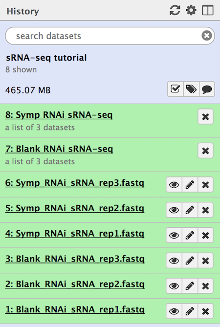
Build a dataset list for both sets (
BlankandSymp) of replicate FASTQ files
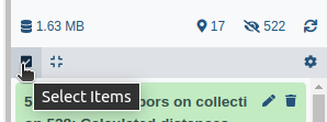
- Click on galaxy-selector Select Items at the top of the history panel
- Check all the datasets in your history you would like to include
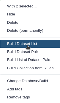
Click n of N selected and choose Advanced Build List
You are in collection building wizard. Choose Flat List and click ‘Next’ button at the right bottom corner.
Double clcik on the file names to edit. For example, remove file extensions or common prefix/suffixes to cleanup the names.
- Enter a name for your collection
- Click Build to build your collection
- Click on the checkmark icon at the top of your history again
Import the remaining files from Zenodo or from the data library (ask your instructor)
https://zenodo.org/record/826906/files/dm3_transcriptome_Tx2Gene_downsampled.tab.gz
https://zenodo.org/record/826906/files/dm3_transcriptome_sequences_downsampled.fa.gz
https://zenodo.org/record/826906/files/dm3_miRNA_hairpin_sequences.fa.gz
https://zenodo.org/record/826906/files/dm3_rRNA_sequences.fa.gz
- Set the datatype of the annotation file to tab and assign the Genome as dm3
- Set the datatype of the reference files to fasta and assign the Genome as dm3


Read quality checking
Read quality scores (phred scores) in FASTQ-formatted data can be encoded by one of a few different encoding schemes. Most Galaxy tools assume that input FASTQ files are using the Sanger/Illumina 1.9 encoding scheme. If the input FASTQ files are using an alternate encoding scheme, then some tools will not interpret the quality score encodings correctly. It is good practice to confirm the quality encoding scheme of your data and then convert to Sanger/Illumina 1.9, if necessary. We can check the quality encoding scheme using the FastQC tool (further described in the NGS-QC tutorial).
Hands On: Quality checking
- Run FastQC tool on the
Blankcollection
- param-collection “Short read data from your current history”:
Blankcollection
- Click on param-collection Dataset collection in front of the input parameter you want to supply the collection to.
- Select the collection you want to use from the list
- Run FastQC tool for the Symplekin RNAi dataset collection
Inspect the FastQC tool reports
Question
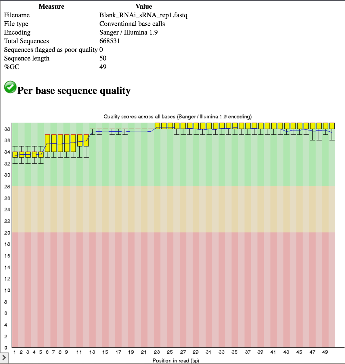
- What quality score encoding scheme is being used for each sample?
- What is the read length for each sample?
What does the base/read quality look like for each sample?
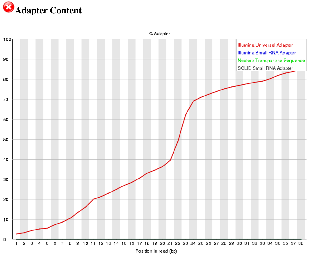
Are there any adaptors present in these reads? Which one(s)?
- All samples use the Illumina 1.9 quality encoding scheme, so we do not need to convert.
- All samples have a read length of 50 nt.
- The base quality across the entire length of the reads is good (phred score > 28 for the most part).
- Yes, the “Illumina Universal Adapter” is present.
Hands On: FormattingIf your data are not in Sanger / Illumina 1.9 format:
- FASTQ Groomer tool on each collection
- param-collection “File to groom”: input collection
- “Input FASTQ quality scores type”:
Illumina 1.3-1.7- Check that the format is fastqsanger instead of fastq
If your data are already in Sanger / Illumina 1.9 format:
Change the datatype to
fastqsanger
- Click on the galaxy-pencil pencil icon for the dataset to edit its attributes
- In the central panel, click galaxy-chart-select-data Datatypes tab on the top
- In the galaxy-chart-select-data Assign Datatype, select
fastqsangerfrom “New Type” dropdown
- Tip: you can start typing the datatype into the field to filter the dropdown menu
- Click the Save button
Go back to the FastQC tool and scroll down to the “Adapter Content” section. You can see that Illumina Universal Adapters are present in >80% of the reads. The next step is to remove these artificial adaptors because they are not part of the biological sRNAs. If a different adapter is present, you can update the Adapter sequence to be trimmed off in the Trim Galore! tool step described below.
Adaptor trimming
sRNA-seq library preparation involves adding an artificial adaptor sequence to both the 5’ and 3’ ends of the small RNAs. While the 5’ adaptor anchors reads to the sequencing surface and thus are not sequenced, the 3’ adaptor is typically sequenced immediately following the sRNA sequence. In the example datasets here, the 3’ adaptor sequence is identified as the Illumina Universal Adapter, and needs to be removed from each read before aligning to a reference. We will be using the Galaxy tool Trim Galore! tool which implements the cutadapt tool for adapter trimming.
Hands On: Adaptor trimming
- Trim Galore! tool on each collection of FASTQ read files to remove Illumina adapters from the 3’ ends of reads with the following parameters:
- “Is this library paired- or single-end”:
Single-end
- param-collection “Reads in FASTQ format?”:
Blankcollection- “Adapter sequence to be trimmed”:
Illumina universal- “Trim Galore! advanced settings”:
Full parameter list
- “Trim low-quality ends from reads in addition to adapter removal”:
0- “Overlap with adapter sequence required to trim a sequence”:
6- “Discard reads that became shorter than length N”:
12- “Generate a report file”:
Yes- Trim Galore! tool: Repeat for the Symplekin RNAi dataset collection
We don’t want to trim for quality because the adapter-trimmed sequences represent a full small RNA molecule, and we want to maintain the integrity of the entire molecule. We increase the minimum read length required to keep a read because small RNAs can potentially be shorter than 20 nt (the default value). We can check out the generated report file for any sample and see the command for the tool, a summary of the total reads processed and number of reads with an adapter identified, and histogram data of the length of adaptor trimmed. We also see that a very small percentage of low-quality bases have been trimmed
Hands On: Adaptor trimming check
- FastQC tool on each collection of trimmed FASTQ read files to assess whether adapters were successfully removed.
Inspect the FastQC tool reports
Question
- What is the read length?
- Are there any adaptors present in these reads? Which one(s)?
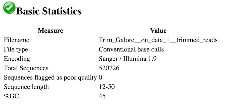
- The read lengths range from 12 to 50 nt after trimming.
- No, Illumina Universal Adaptors are no longer present. No other adapters are present.
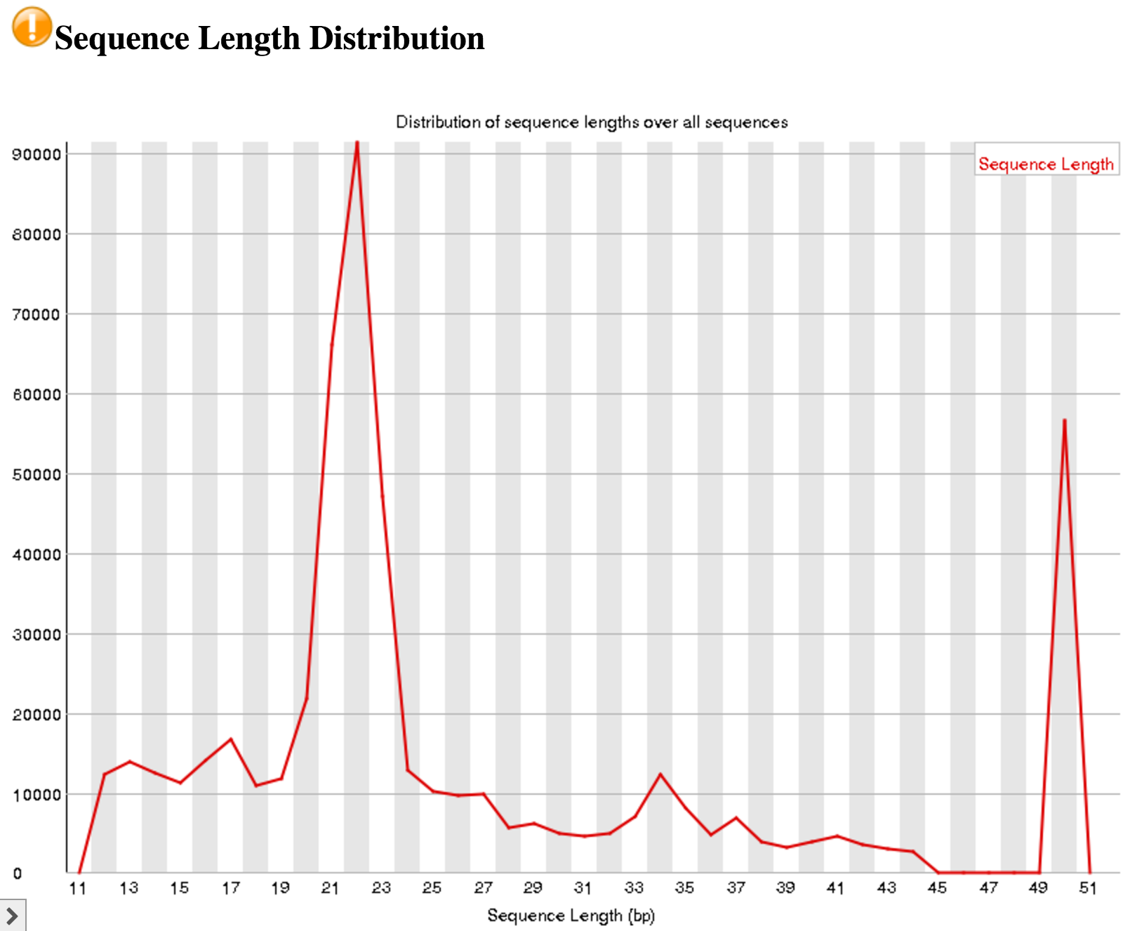
An interesting thing to note from our FastQC tool results is the Sequence Length Distribution results. While many RNA-seq experiments have normal distribution of read lengths, an unusual spike at 22nt is observed in our data. This spike represents the large set of endogenous siRNAs that occur in the cell line used in this study, and is actually confirmation that our dataset captures the biological molecule we are interested in.
Now that we have converted to fastqsanger format and trimmed our reads of the Illumina Universal Adaptors, we will align our trimmed reads to reference Drosophila rRNA and miRNA sequences (dm3) to remove these artifacts. Interestingly, Drosophila have a short 2S rRNA sequence that is 30nt long and typically co-migrates with sRNA populations during gel electrophoresis. rRNAs make up a very large proportion of all non-coding RNAs, and thus need to be removed. Oftentimes, experimental approaches can be utilized to deplete or avoid capture of rRNAs, but these methods are not always 100% efficient. We also want to remove any miRNA sequences, as these are not relevant to our analysis. After removing rRNA and miRNA reads, we will analyze the remaining reads, which may be siRNA or piRNA sequences.
Hierarchical read alignment to remove rRNA/miRNA reads
To first identify rRNA-originating reads (which we are not interested in in this case), we will align the reads to a reference set of rRNA sequences using HISAT2 tool, an accurate and fast tool for aligning reads to a reference.
Hands On: Hierarchical alignment to rRNA and miRNA reference sequences
- HISAT2 tool on each collection of trimmed reads to align to reference rRNA sequences with the following parameters
- “Source for the reference genome to align against”:
Use a genome from history
- param-file “Select the reference genome”:
Dmel_rRNA_sequences.fa- “Is this a single or paired library?”:
Single-end
- param-collection “FASTA/Q file”: output of Trim Galore! tool for
Blankcollection- “Specify strand-specific information”:
Forward (F)- HISAT2 tool: Repeat for the Symplekin RNAi dataset collection
We now need to extract the unaligned reads from the output BAM file for aligning to reference miRNA sequences. We can do this by using the Filter SAM or BAM, output SAM or BAM tool to obtain reads with a bit flag = 4 (meaning the read is unaligned) and then converting the filtered BAM file to FASTQ format with the Convert from BAM to FastQ tool.
Hands On: Hierarchical alignment to rRNA and miRNA reference sequences (2)
- Filter SAM or BAM, output SAM or BAM tool on collection of HISAT2 output BAM files with the following parameters
- param-collection “SAM or BAM file to filter”: output of HISAT2 tool for
Blankcollection- “Filter on bitwise flag”:
Yes
- “Only output alignments with all of these flag bits set”:
The read in unmapped- Filter SAM or BAM, output SAM or BAM tool: Repeat for the Symplekin RNAi dataset collection
- Convert from BAM to FastQ tool on each collection of filtered HISAT2 output BAM files with the following parameters:
- param-collection “Convert the following BAM file to FASTQ”: output of Filter SAM or BAM tool for
Blankcollection- Convert from BAM to FastQ tool: Repeat for the Symplekin RNAi dataset collection
Next we will align the non-rRNA reads to a known set of miRNA hairpin sequences to identify miRNA reads.
Hands On: Hierarchical alignment to rRNA and miRNA reference sequences (3)
- HISAT2 tool on each collection of filtered HISAT2 output FASTQ files to align non-rRNA reads to reference miRNA hairpin sequences using the following parameters:
- “Source for the reference genome to align against”:
Use a genome from history
- param-file “Select the reference genome”:
Dmel_miRNA_sequences.fa- “Is this a single or paired library?”:
Single-end
- param-collection “FASTA/Q file”: output of Convert from BAM to FastQ tool for
Blankcollection- “Specify strand-specific information”:
Forward (F)- HISAT2 tool: Repeat for the Symplekin RNAi dataset collection
For this tutorial we are not interested in miRNA reads, so we need to extract unaligned reads from the output BAM files. To do this, repeat the Filter SAM or BAM, output SAM or BAM tool steps for each dataset collection. Finally, rename the converted FASTQ files something meaningful (e.g. “non-r/miRNA control RNAi sRNA-seq”).
In some instances, miRNA-aligned reads are the desired output for downstream analyses, for example, if we are investigating how loss of key miRNA pathway components affect levels of pre-miRNA and mature miRNAs. In this case, the BAM output of HISAT2 can directly be used in subsequent tools as it contains the subset of reads aligned to miRNA sequences.
Small RNA subclass distinction
In Drosophila, non-miRNA small RNAs are typically divided into two major groups: endogenous siRNAs which are 20-22nt long and piRNAs which are 23-29nt long. We want to analyze these sRNA subclasses independently, so next we are going to filter the non-r/miRNA reads based on length using the Manipulate FASTQ tool tool.
Hands On: Extract subclasses
- Manipulate FASTQ tool on each collection of non-r/miRNA reads to identify siRNAs (20-22nt) using the following parameters.
- param-collection “FASTQ File”: output of last HISAT tool for
Blankcollection- Click on “Insert Match Reads”
- In “1: Match Reads”
- “Match Reads by”:
Sequence Content
- “Match by”:
^.{12,19}$|^.{23,50}$- Click on “Manipulate Reads”
- In “1: Manipulate Reads”
- “Manipulate Reads on”:
Miscellaneous actions
- “Miscellaneous Manipulation Type”:
Remove Read- Manipulate FASTQ tool: Repeat for the Symplekin RNAi dataset collection
- Rename each resulting dataset collection something meaningful (i.e. “blank RNAi - siRNA reads (20-22nt)”)
The regular expression in the Match by parameter tells the tool to identify sequences that are length 12-19 or 23-50 (inclusive), and the Miscellaneous Manipulation Type parameter tells the tool to remove these sequences. What remains are sequences of length 20-22nt. We will now repeat these steps to identify sequences in the size-range of piRNAs (23-29nt).
Hands On: Extract subclasses
- Manipulate FASTQ tool: Run
Manipulate FASTQon each collection of non-r/miRNA reads to identify sequences in the size-range of piRNAs (23-29nt)
- param-collection “FASTQ File”: output of last HISAT tool for
Blankcollection- Click on “Insert Match Reads”
- In “1: Match Reads”
- “Match Reads by”:
Sequence Content
- “Match by”:
^.{12,22}$|^.{30,50}$- Click on “Manipulate Reads”
- In “1: Manipulate Reads”
- “Manipulate Reads on”:
Miscellaneous actions
- “Miscellaneous Manipulation Type”:
Remove Read- Manipulate FASTQ tool: Repeat for the Symplekin RNAi dataset collection
- Rename each resulting dataset collection something meaningful (i.e. “blank RNAi - piRNA reads (23-29nt)”)
Hands On: Check the read length
- FastQC tool: Run
FastQCon each collection of siRNA and piRNA read files to confirm the correct read lengths.
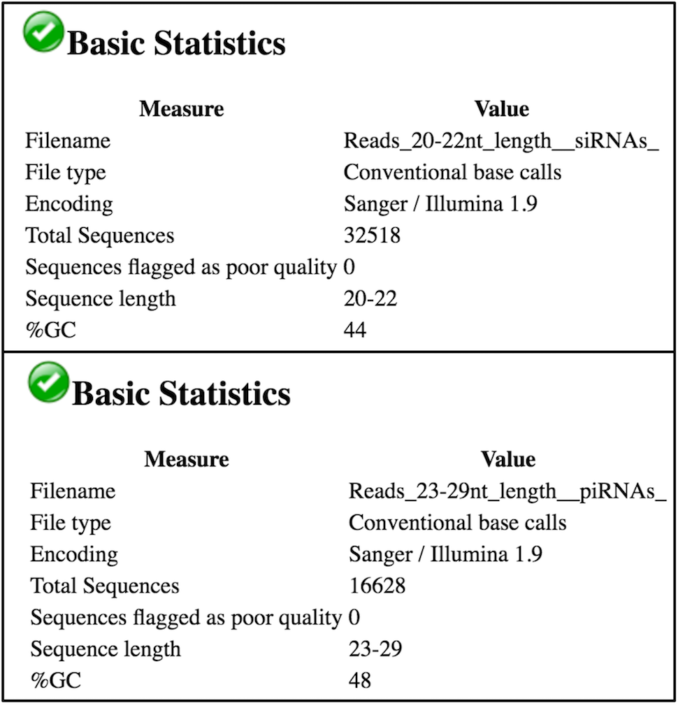
We see in the above image (for Blank RNAi, replicate 3) that we have ~32k reads that are 20-22nt long in our Reads_20-22_nt_length_siRNAs file and ~16k reads that are 23-29nt long in our Reads_23-29_nt_length_piRNAs file, as expected. Given that we had ~268k trimmed reads in the Blank RNAi replicate 3 file, siRNAs represent ~12.1% of the reads and piRNAs represent ~6.2% of the reads in this experiment. There is no distinct peak in the piRNA range (you can find the example of the real piRNA profile in Figure 1 from Colin D. Malone et al, 2009.
The next step in our analysis pipeline is to identify which RNA features - e.g. protein-coding mRNAs, transposable elements - the siRNAs and piRNAs align to. Most fly piRNAs originate from and thus align to transposable elements (TEs) but some also originate from genome piRNA clusters or protein-coding genes. siRNAs are thought to inhibit TE mobility and potentially target mRNAs for degradation via an RNA-interference (RNAi) mechanism. Ultimately, we want to know whether an RNA feature (TE, piRNA cluster, mRNA, etc.) has significantly different numbers of siRNAs or piRNAs targeting it. To determine this, we will use Salmon tool to simultaneously align and quantify siRNA reads against known target sequences to estimate siRNA abundance per target. For the remainder of the tutorial we will be focusing on siRNAs, but similar approaches can be done for piRNAs, miRNAs, or any other subclass of small, non-coding RNAs.
siRNA abundance estimation
We want to identify which siRNAs are differentially abundance between the blank and Symplekin RNAi conditions. To do this we will implement a counting approach using Salmon tool to quantify siRNAs per RNA feature. Specifically, we will analyzing mRNA and TE elements by counting siRNAs against a FASTA file of transcript sequences, not the reference genome. This approach is especially useful in this case because we are interested in TEs, which occur at many copies (100s - 1000s) in the genome, and thus will result in multiple alignments if we align to the genome with a tool like HISAT2 tool. Further, we will be counting abundance of siRNAs that align sense or antisense to an RNA feature independently, as opposite sense alignments are correlated with unique downstream silencing effects. Then, we will provide this information to DESeq2 tool to generate normalized counts and significance testing for differential abundance of siRNAs per feature.
Hands On: siRNA abundance estimation
- Salmon tool on each collection of siRNA reads (20-22nt) to quantify the abundance of antisense siRNAs at relevant targets
- “Select a reference transcriptome from your history or use a built-in index?”:
Use one from the history
- param-file “Select the reference transcriptome”:
the reference mRNA and TE fasta file- “The size should be odd number”:
19- “Is this library mate-paired?”:
Single-end
- param-collection “FASTQ/FASTA file”: collection with the Blank RNAi siRNA (20-22nt) reads
- “Specify the strandedness of the reads”:
read 1 (or single-end read) comes from the reverse strand (SR)- In “Additional Options”
- “Incompatible Prior”:
0- Salmon tool: Repeat for the Symplekin RNAi siRNAs (20-22nt) reads dataset collection
- Salmon tool: Repeat on each collection of siRNA reads (20-22nt) to quantify the abundance of sense siRNAs at relevant targets by changing the following parameters:
- “Specify the strandedness of the reads”:
read 1 (or single-end read) comes from the forward strand (SF)
The output of Salmon tool includes a table of RNA features, estimated counts, transcripts per million, and feature length. We will be using the TPM quantification column as input to DESeq2 tool in the next section.
siRNA differential abundance testing
DESeq2 tool is a great tool for differential expression analysis, but we also employ it here for estimation of abundance of reads targeting each of our RNA features. As input, DESeq2 tool can take transcripts per million (TPM) counts produced by Salmon tool for each feature. TPMs are estimates of the relative abundance of a given transcript in units, and analogously can be used here to quantify siRNAs that align either sense or antisense to transcripts.
Hands On: siRNA differential abundance testing
- DESeq2 tool to test for differential abundance of antisense siRNAs at mRNA and TE features using the following parameters:
- In “Factor”:
- In “1: Factor”
- “Specify a factor name”:
RNAi- In “Factor level”:
- In “1: Factor level”:
- “Specify a factor level”:
Symplekin- param-collection “Counts file(s)”: the Symplekin RNAi siRNA counts from reverse strand (SR) collection
- In “2: Factor level”:
- “Specify a factor level”:
RNAi- param-collection “Counts file(s)”: the Symplekin RNAi siRNA counts from reverse strand (SR)
- “Choice of Input data”:
TPM values (e.g. from sailfish and salmon)
- “Program used to generate TPMs”:
Salmon- “Gene mapping format”:
Transcript-ID and Gene-ID mapping file
- param-file “Tabular file with Transcript - Gene mapping”:
reference tx2g (transcript to gene) file(available through zenodo link)- “Output normalized counts table”:
Yes- DESeq2 tool for the sense siRNAs at mRNA and TE features:
- In “Factor”:
- In “1: Factor”
- “Specify a factor name”:
RNAi- In “Factor level”:
- In “1: Factor level”:
- “Specify a factor level”:
Symplekin- param-collection “Counts file(s)”: the Symplekin RNAi siRNA counts from forward strand (SF)
- In “2: Factor level”:
- “Specify a factor level”:
RNAi- param-collection “Counts file(s)”: the Symplekin RNAi siRNA counts from forward strand (SF)
- “Choice of Input data”:
TPM values (e.g. from sailfish and salmon)
- “Program used to generate TPMs”:
Salmon- “Gene mapping format”:
Transcript-ID and Gene-ID mapping file
- param-file “Tabular file with Transcript - Gene mapping”:
reference tx2g (transcript to gene) file(available through zenodo link)- “Output normalized counts table”:
Yes- Filter tool to extract features with a significantly different antisense siRNA abundance (adjusted p-value less than 0.05).
- param-file “Filter”: Select the
DESeq2result file from testing antisense (SR) siRNA abundances- “With following condition”:
c7<0.05- Filter tool for the sense siRNAs at mRNA and TE features:
- param-file “Filter”: Select the
DESeq2result file from testing sense (SF) siRNA abundances- “With following condition”:
c7<0.05
QuestionHow many features have a significant difference in antisense and sense siRNA abundance in the Symplekin RNAi condition?
There are 87 antisense and 15 sense features that have significanlty different siRNA abundances.
For more information about DESeq2 and its outputs, have a look at DESeq2 documentation.
Visualization
Coming soon!
Conclusion
Analysis of small RNAs is a complicated and intricate process due to the diversity in characteristics, functionality, and nuances of small RNA subclasses. The goal of this tutorial is to introduce you to a common small RNA workflow that specifically identifies changes in endogenous siRNA abundances that target protein-coding mRNAs and transposable elements. The steps presented here can be rearranged and modified based on small RNA features of specific systems and the needs of the user.
Small RNA analysis (general) pipeline
You've Finished the Tutorial
Key points
Analysis of small RNAs is complex due to the diversity of small RNA subclasses.
Both alignment to references and transcript quantification approaches are useful for small RNA-seq analyses.
Frequently Asked Questions
Have questions about this tutorial? Have a look at the available FAQ pages and support channelsUseful literature
Further information, including links to documentation and original publications, regarding the tools, analysis techniques and the interpretation of results described in this tutorial can be found here.
Feedback
Did you use this material as an instructor? Feel free to give us feedback on how it went.
Did you use this material as a learner or student? Click the form below to leave feedback.

Citing this Tutorial
- Mallory Freeberg, Differential abundance testing of small RNAs (Galaxy Training Materials). https://training.galaxyproject.org/training-material/topics/transcriptomics/tutorials/srna/tutorial.html Online; accessed TODAY
- Hiltemann, Saskia, Rasche, Helena et al., 2023 Galaxy Training: A Powerful Framework for Teaching! PLOS Computational Biology 10.1371/journal.pcbi.1010752
- Batut et al., 2018 Community-Driven Data Analysis Training for Biology Cell Systems 10.1016/j.cels.2018.05.012
Congratulations on successfully completing this tutorial!@misc{transcriptomics-srna, author = "Mallory Freeberg", title = "Differential abundance testing of small RNAs (Galaxy Training Materials)", year = "", month = "", day = "", url = "\url{https://training.galaxyproject.org/training-material/topics/transcriptomics/tutorials/srna/tutorial.html}", note = "[Online; accessed TODAY]" } @article{Hiltemann_2023, doi = {10.1371/journal.pcbi.1010752}, url = {https://doi.org/10.1371%2Fjournal.pcbi.1010752}, year = 2023, month = {jan}, publisher = {Public Library of Science ({PLoS})}, volume = {19}, number = {1}, pages = {e1010752}, author = {Saskia Hiltemann and Helena Rasche and Simon Gladman and Hans-Rudolf Hotz and Delphine Larivi{\`{e}}re and Daniel Blankenberg and Pratik D. Jagtap and Thomas Wollmann and Anthony Bretaudeau and Nadia Gou{\'{e}} and Timothy J. Griffin and Coline Royaux and Yvan Le Bras and Subina Mehta and Anna Syme and Frederik Coppens and Bert Droesbeke and Nicola Soranzo and Wendi Bacon and Fotis Psomopoulos and Crist{\'{o}}bal Gallardo-Alba and John Davis and Melanie Christine Föll and Matthias Fahrner and Maria A. Doyle and Beatriz Serrano-Solano and Anne Claire Fouilloux and Peter van Heusden and Wolfgang Maier and Dave Clements and Florian Heyl and Björn Grüning and B{\'{e}}r{\'{e}}nice Batut and}, editor = {Francis Ouellette}, title = {Galaxy Training: A powerful framework for teaching!}, journal = {PLoS Comput Biol} }
You can use Ephemeris's
shed-tools installcommand to install the tools used in this tutorial.shed-tools install [-g GALAXY] [-a API_KEY] -t <(curl https://training.galaxyproject.org/training-material/api/topics/transcriptomics/tutorials/srna/tutorial.json | jq .admin_install_yaml -r)Alternatively you can copy and paste the following YAML
---
install_tool_dependencies: true
install_repository_dependencies: true
install_resolver_dependencies: true
tools:
- name: salmon
  owner: bgruening
  revisions: 53e9709776a0
  tool_panel_section_label: RNA Analysis
  tool_shed_url: https://toolshed.g2.bx.psu.edu/
- name: trim_galore
  owner: bgruening
  revisions: 1bfc7254232e
  tool_panel_section_label: FASTA/FASTQ
  tool_shed_url: https://toolshed.g2.bx.psu.edu/
- name: fastq_manipulation
  owner: devteam
  revisions: bb07615a5b6a
  tool_panel_section_label: FASTA/FASTQ
  tool_shed_url: https://toolshed.g2.bx.psu.edu/
- name: fastqc
  owner: devteam
  revisions: 3fdc1a74d866
  tool_panel_section_label: FASTA/FASTQ
  tool_shed_url: https://toolshed.g2.bx.psu.edu/
- name: samtool_filter2
  owner: devteam
  revisions: dc6ff68ea5e8
  tool_panel_section_label: SAM/BAM
  tool_shed_url: https://toolshed.g2.bx.psu.edu/
- name: bedtools
  owner: iuc
  revisions: c78cf6fe3018
  tool_panel_section_label: BED
  tool_shed_url: https://toolshed.g2.bx.psu.edu/
- name: deseq2
  owner: iuc
  revisions: 24a09ca67621
  tool_panel_section_label: RNA Analysis
  tool_shed_url: https://toolshed.g2.bx.psu.edu/
- name: hisat2
  owner: iuc
  revisions: 1eb21dccc2fa
  tool_panel_section_label: Mapping
  tool_shed_url: https://toolshed.g2.bx.psu.edu/