Network analysis with Heinz
| Author(s) |
|
| Reviewers |
|
OverviewQuestions:
Objectives:
Which pathways are potentially contributing to dental caries?
Requirements:
Network Analysis of metatranscriptomics data using Heinz in Galaxy to pinpoint the optimal scoring subnetwork.
- Introduction to Galaxy Analyses
- slides Slides: Quality Control
- tutorial Hands-on: Quality Control
- slides Slides: Mapping
- tutorial Hands-on: Mapping
Time estimation: 1 hour 30 minutesSupporting Materials:Published: Oct 11, 2018Last modification: May 18, 2023License: Tutorial Content is licensed under Creative Commons Attribution 4.0 International License. The GTN Framework is licensed under MITpurl PURL: https://gxy.io/GTN:T00293rating Rating: 4.3 (0 recent ratings, 4 all time)version Revision: 16
Overview
The human microbiome plays a key role in health and disease. Thanks to comparative metatranscriptomics, the cellular functions that are deregulated by the microbiome in disease can now be computationally explored. Unlike gene-centric approaches, pathway-based methods provide a systemic view of such functions; however, they typically consider each pathway in isolation and in its entirety. They can therefore overlook the key differences that (i) span multiple pathways, (ii) contain bidirectionally deregulated components, (iii) are confined to a pathway region. To capture these properties, computational methods that reach beyond the scope of predefined pathways are needed.
In this tutorial, we will perform a network analysis using Heinz (GitHub, publication) in Galaxy. The data comes from the study May et al., and we will reproduce some of the computational steps from this study with simplified data and parameters to speed up the analysis for the purposes of this tutorial.
AgendaIn this tutorial, we will cover:
Comment: Results may varyYour results may be slightly different from the ones presented in this tutorial due to differing versions of tools, reference data, external databases, or because of stochastic processes in the algorithms.
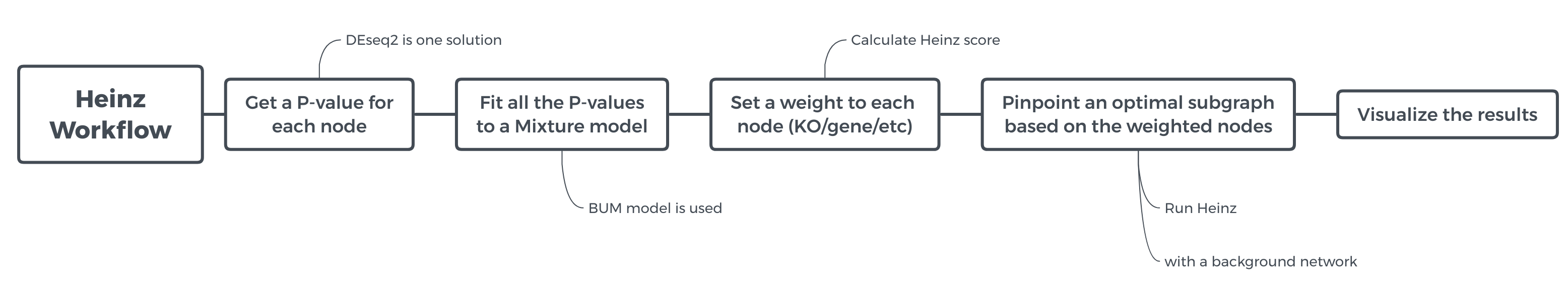
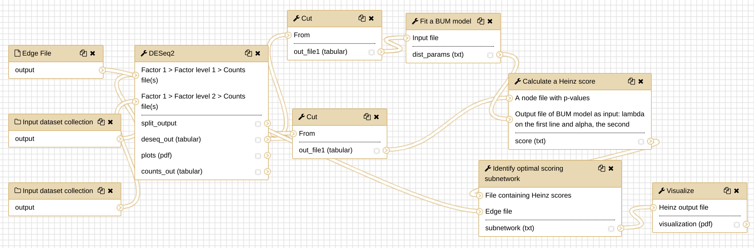
In this tutorial, we will run the Heinz workflow step by step to understand how each step works. To get an overview of what this workflow does and what kind of calculation is involved, view the flowchart below.
Obtaining and preparing data 
The study May et al. includes the computation steps starting from the raw RNAseq datasets. The operations that processed raw data into the interpreted data are beyond the scope of this tutorial. To learn that, please refer to the relevant topics in the Galaxy training material. In this tutorial, we start with the interpreted data, which are KO (KEGG Orthology) count data. All the data needed for this tutorial are available from Zenodo.
KOs are organism-independent identifiers that group together proteins of similar biochemical functions. It is a term specific to KEGG database. It is a group concept, similar to the concept “pathway”, which includes a bunch of molecules and their interactions. Take a random line in our dataset, “K01369 7” as an example, the first column represents the KO ID, and the second column — the numeric value is the KO counts. If we understand it by the face value, it is 7 protein molecules that are counted from our dataset as this KO “K01369”; but we usually mingle proteins with genes because we often assume that each protein corresponds to a gene, so it can be understood as 7 genes. Now we are working on the microbial RNAseq data, and the assumption is also used subconsciously.
Understanding our input data
According to the study May et al., dental caries (DC) dataset in this tutorial came from an experiment that comprised of supragingival plaque samples collected from all dental surfaces of 36 individuals who had either a caries-positive (disease) or a caries-negative (health) oral profile. Each of the 36 samples was sequenced, pre-processed and transformed into KO counts. We will use these count data as the starting point to perform the network analysis.
Comment: Dataset detailsThe count data of the 36 samples are separated into 36 files, organized into two groups: ‘CP’ (caries-positive) and ‘CN’ (caries-negative).
Importing the data into Galaxy
After knowing what our input data are like, let’s get them into Galaxy history:
Hands On: Obtaining our data
Make sure we have an empty Galaxy history. Give it a sensible name.
To create a new history simply click the new-history icon at the top of the history panel:
- Click on galaxy-pencil (Edit) next to the history name (which by default is “Unnamed history”)
- Type the new name
- Click on Save
- To cancel renaming, click the galaxy-undo “Cancel” button
If you do not have the galaxy-pencil (Edit) next to the history name (which can be the case if you are using an older version of Galaxy) do the following:
- Click on Unnamed history (or the current name of the history) (Click to rename history) at the top of your history panel
- Type the new name
- Press Enter
- Upload Disease Dataset
- Open the file upload menu
- Click on Collection tab
- Click on the Paste/Fetch data button
- Copy the Zenodo links for the Disease Datasets
https://zenodo.org/record/1344105/files/2241_CP_DZ_PairTo_2242.txt https://zenodo.org/record/1344105/files/2126_CP_MZ_PairTo_2125.txt https://zenodo.org/record/1344105/files/2991_CP_DZ_PairTo_2992.txt https://zenodo.org/record/1344105/files/2931_CP_DZ_PairTo_2930.txt https://zenodo.org/record/1344105/files/2284_CP_DZ_PairTo_2283.txt https://zenodo.org/record/1344105/files/2125_CP_MZ_PairTo_2126.txt https://zenodo.org/record/1344105/files/4131_CP_DZ_PairTo_4132.txt https://zenodo.org/record/1344105/files/2954_CP_DZ_PairTo_2955.txt https://zenodo.org/record/1344105/files/2170_CP_MZ_PairTo_2169.txt https://zenodo.org/record/1344105/files/2955_CP_DZ_PairTo_2954.txt https://zenodo.org/record/1344105/files/2011_CP_DZ_PairTo_2012.txt https://zenodo.org/record/1344105/files/2012_CP_DZ_PairTo_2011.txt https://zenodo.org/record/1344105/files/2269_CP_DZ_PairTo_2270.txt https://zenodo.org/record/1344105/files/3215_CP_MZ_PairTo_3214.txt https://zenodo.org/record/1344105/files/2354_CP_DZ_PairTo_2355.txt https://zenodo.org/record/1344105/files/3306_CP_DZ_PairTo_3307.txt https://zenodo.org/record/1344105/files/2061_CP_DZ_PairTo_2062.txt https://zenodo.org/record/1344105/files/2355_CP_DZ_PairTo_2354.txt https://zenodo.org/record/1344105/files/2242_CP_DZ_PairTo_2241.txt- Click on Start to Upload the files
- Click Build once upload has completed
- Enter Name:
CP- Click Create list to make the collection
- Upload control (healthy) datasets
- Repeat the previous steps with the samples from healthy individuals:
https://zenodo.org/record/1344105/files/2310_CN_DZ_PairTo_2309.txt https://zenodo.org/record/1344105/files/2062_CN_DZ_PairTo_2061.txt https://zenodo.org/record/1344105/files/2191_CN_MZ_PairTo_2192.txt https://zenodo.org/record/1344105/files/2052_CN_MZ_PairTo_2051.txt https://zenodo.org/record/1344105/files/2051_CN_MZ_PairTo_2052.txt https://zenodo.org/record/1344105/files/2192_CN_MZ_PairTo_2191.txt https://zenodo.org/record/1344105/files/2234_CN_DZ_PairTo_2233.txt https://zenodo.org/record/1344105/files/2233_CN_DZ_PairTo_2234.txt https://zenodo.org/record/1344105/files/2270_CN_DZ_PairTo_2269.txt https://zenodo.org/record/1344105/files/2225_CN_MZ_PairTo_2226.txt https://zenodo.org/record/1344105/files/4132_CN_DZ_PairTo_4131.txt https://zenodo.org/record/1344105/files/2309_CN_DZ_PairTo_2310.txt https://zenodo.org/record/1344105/files/2992_CN_DZ_PairTo_2991.txt https://zenodo.org/record/1344105/files/3214_CN_MZ_PairTo_3215.txt https://zenodo.org/record/1344105/files/2169_CN_MZ_PairTo_2170.txt https://zenodo.org/record/1344105/files/2930_CN_DZ_PairTo_2931.txt https://zenodo.org/record/1344105/files/3307_CN_DZ_PairTo_3306.txt- Name this collection:
CNQuestion
- How many samples do you have in our disease collection (CP)? How many healthy samples (CN)?
- How many columns in each file? What are these columns?
- You should have 19 samples in the disease collection (CP), and 17 in the negative collection (CN).
- There are two columns, one is the KO IDs, the other is the count.

Dataset collections enables us to easily run tools on multiple datasets at once, you probably have done that in the file upload menu using the
Collectiontab. If not, you can still create dataset collections manually.Hands On: Manually organizing our data into a collectionIf you have all the datasets in the history, but they are not organized into a collection yet, you can follow these steps to create a collection:
Click on the checkmark icon at top of your history.
Select all the files whose name contains
CP, then click on n of N selected and select Build Dataset List from the dropdown menu.In the next dialog window, you need to give a name, here we just set it to
CP, then click Create list.Redo the Step 2, 3 for CN, set the name of the data list as ‘CN’.
Differential Expression Analysis (DEA) by DESeq2
What is differential expression analysis?
Comment: A definitionThe definition of differential expression analysis given by EBI means taking the normalised read count data and performing statistical analysis to discover quantitative changes in expression levels between experimental groups. For example, we use statistical testing to decide whether, for a given gene, an observed difference in read counts is significant, that is, whether it is greater than what would be expected just due to natural random variation.
In principle, DEA is a causal analysis; but in reality, it is hampered by the complexity of the experimental situation and measurement. Back to our datasets, CP and CN, they are from two experimental groups. By DEA, we hope to pinpoint the candidate genes relevant to dental caries first, then we will use Heinz to infer the related pathways.
Which tools are available for DEA?
There are a few canned tools commonly used for DEA, like Limma and DESeq2. If you are interested, you may look up the pros and cons of each tool. Here we use DESeq2.
Perform Differential Expression Analysis (DEA)
After learning about differential expression analysis, let’s get some hands-on experience.
Hands On: DEA via DESeq2
- DESeq2 tool with the following parameters
- “Specify a factor name”:
dental_caries(under1: Factor)- “Specify a factor level”: to
CP(under1: Factor level)
- param-files “Counts file(s)”:
CP(collection)- “Specify a factor level”:
CN(under2: Factor level)
- param-files “Counts file(s)”:
CN(collection)- “Files have header”:
No- “Visualising the analysis results”:
No- Leave all other parameters to the default settings
It takes a few minutes to finish DESseq2. After the analysis is finished, have a look at the file, it should look like something this:
GeneID  Base mean   log2(FC)	        StdErr	            Wald-Stats	        P-value	                P-adj
K15661  55.0733128361562    2.49892393773464	0.508475451930939	4.91454194739384	8.89902710599613e-07	0.00491938218419466
K15666  48.4532561772761    2.22805029428311	0.493391718412049	4.51578372951607	6.30830206230236e-06	0.00820667379798327
K10213  25.1966742274619    -2.45624670858868	0.550895251183889	-4.45864563782342	8.24791475064012e-06	0.00820667379798327
K03732  563.63634258472 -1.41961721984814	0.316992240900184	-4.47839737596338	7.52055094378821e-06	0.00820667379798327
K01792  112.923146882195    -1.26925892659617	0.285732234964578	-4.44212717810268	8.90738834802815e-06	0.00820667379798327
Fit a BUM model (a mixture model)
From a statistical point of view, p-values are uniformly distributed under null hypothesis; in other words, under alternative hypothesis, the noise component (which holds under null hypothesis) will be adequately modeled by a uniform distribution. With this knowledge, we can fit these p-values to a mixture model (BUM model), as the figure below shows.
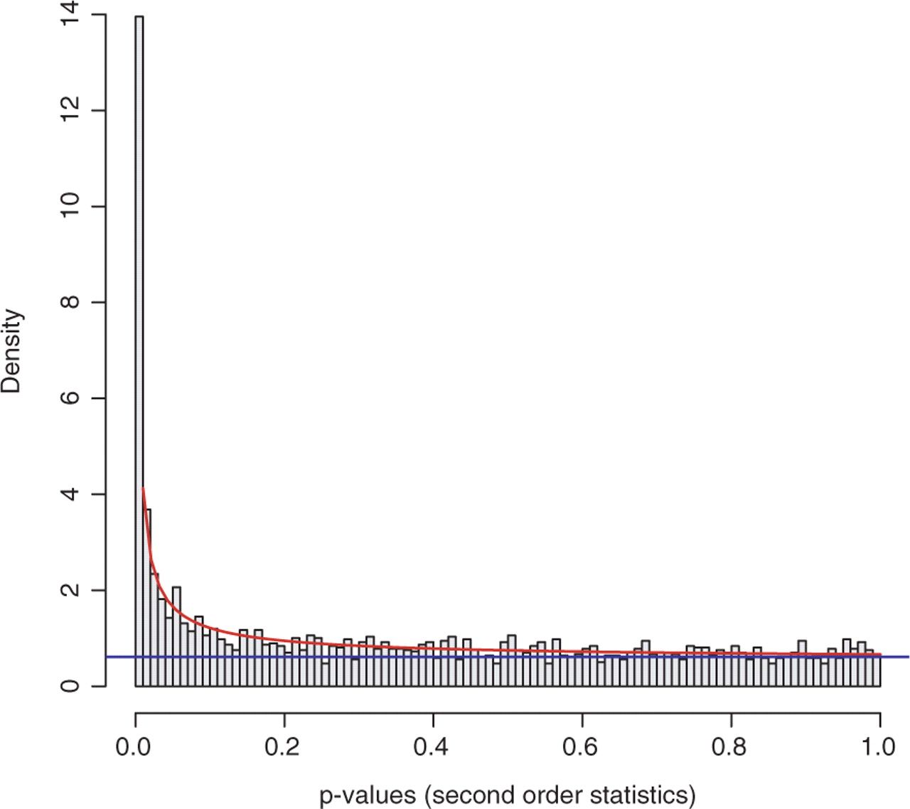
Comment: Why do we need a mixture model?To avoid making this tutorial sound like a math class, let’s focus on the philosophy of using a statistical model. In the graph above, we have visualized the p-values; those bins have some shapes; by viewing the figure, it is possible for us to cherrypick the data points (KO) with mesh eyes, but it must be tedious and boring, nobody wants to spend a few days on doing this. In this situation, computers come into play; however, unlike humans, computers cannot understand the graph but mathematical formulas, that’s why we need to fix the data into a statistical model (denoted by the red curve and blue line in the graph), which computers can understand easily.
Before fitting to BUM model in Galaxy, we need to prepare the input data for the tool Fit a BUM model, that’s a file that only contains p-values.
Hands On: extract p-values from DESeq2 output
- cut columns from a table tool with the following parameters:
- “Cut columns”:
c6- “Delimited by”: to
TAB- “From”: to the output of DESeq2
Now we can Fit a BUM model:
Hands On: fit the BUM model
- Fit a BUM model tool with the following parameters
- “Input file”: the output of cut
Pinpoint the key pathways with Heinz
After getting the parameters of the BUM model from the last step, we will use Heinz to pinpoint the optimal subnetwork. Then we could look for the key pathways relevant to the subnetwork. Before we continue, let’s figure out what Heinz is actually doing.
Heinz is an algorithm for searching an optimal subnetwork from a bigger network. You may wonder what the network is here. Through the previous steps, we have got a list of identities, that is a list of gene IDs with p-values, which form the nodes of ‘the bigger network’, the relations between the nodes, that is the edges, needs to be obtained from a background network, which represents a pathway relation databases, such as Reactome and STRING. In this tutorial, we only use a small sample background network for demonstration purposes. The background network is represented as edges in a TXT file where each line denotes an edge as follows:
ACTR1B	ACVR2B
ZSWIM9	FOXP3
LGALS4	PRKX
NPTX1	CIAO1
Upload this edge file (hereafter we call it edge file) into the Galaxy instance.
Hands On: Upload edge file
- Upload the edge file from Zenodo
- Open the upload menu
- Choose Paste/Fetch data option
- Paste the URL into the box:
https://zenodo.org/record/1344105/files/edge.txt- Click Start
Calculate Heinz scores
As the first step, we need to calculate a Heinz score for each node, using the BUM model parameters we obtained; meanwhile, we also need to specify an FDR value as input.
Comment: What is an FDR value?FDR is short for false discovery rate, which is a method of conceptualizing the rate of type I errors in null hypothesis testing when conducting multiple comparisons, if you are interested, view the detail in Wikipedia.
For different datasets and problems, we probably need to pick up an FDR value separately. Here we set FDR to 0.11.
Similar to Fit a BUM model, we also need to prepare the input data for the tool Calculate a Heinz score.
QuestionWhat is the requirement of the input data format for Calculate a Heinz score?
In the user interface of the tool “Calculate a Heinz score”, we see that “A node file with p-values” is needed. It should contain two columns delimited by tab, one is KO ID; the other, p-value.
Hands On: extract geneID and p-values from DESeq2 output
- cut columns from a table tool with the following parameters
- “Cut columns”:
c1,c6- “Delimited by”:
TAB- “From”: the output of DESeq2
Hands On: calculate Heinz scores
- Calculate a Heinz score tool with the following parameters
- “A node file with p-values”: the output of the previous cut step
- “FDR value”: to 0.11
- “Choose your input type for BUM parameters”:
The output file of BUM model- “Output file of BUM model as input: lambda on the first line and alpha, the second”: the output of Fit a BUM model
Comment: What is the Heinz score?To figure out this score without reading the formula, we can understand Heinz score in this way. FDR is involved in calculating a p-value threshold and any KO whose p-value is below this threshold is regarded as significant, which means the Heinz score is positive (another calculation in the formula). If we pick a higher FDR value, then we will have a higher p-value threshold, and more KOs are probably regarded as significant. In this situation, we probably have many false positive (those regarded as significant are actually not) on the one hand; on the other hand, Heinz will deliver a bigger subnetwork, which might be exhausting to analyze. Therefore, we need to pick up an FDR value properly.
Run Heinz: pinpoint the optimal subnetwork
After getting Heinz scores, let’s run Heinz program to find the optimal subnetwork from the background network which we mentioned earlier.
Hands On: pinpoint the optimal subnetwork
- Identify optimal scoring subnetwork tool with the following parameters
- “File containing Heinz scores”: the output of Calculate a Heinz score
- “Edge file”: the edge file uploaded
It usually takes a few minutes to get the result, but mind you, for some tasks, it might take a few hours to get a result in practice.
Comment: The running time of the program
- Graph problem is way more complicated than we thought.
- It might take a much longer time for some complicated datasets.
- We can use multiple CPUs to accelerate the computation (for now, this function is not available in Galaxy yet), but, to use that, you can install Heinz directly via Bioconda in a Linux environment.
Visualize the output: visualize the optimal subnetwork
The result we got from the last step is not very human-readable, is it? It is a little painful to understand the Heinz result directly. Therefore we need to visualize the output by making it into graphs.
Hands On: visualize the optimal subnetwork
- Visualize the optimal scoring subnetwork tool with the following parameters
- “Heinz output file”: the output of Identify optimal scoring subnetwork
In this tutorial, you probably get a similar graph to the following:
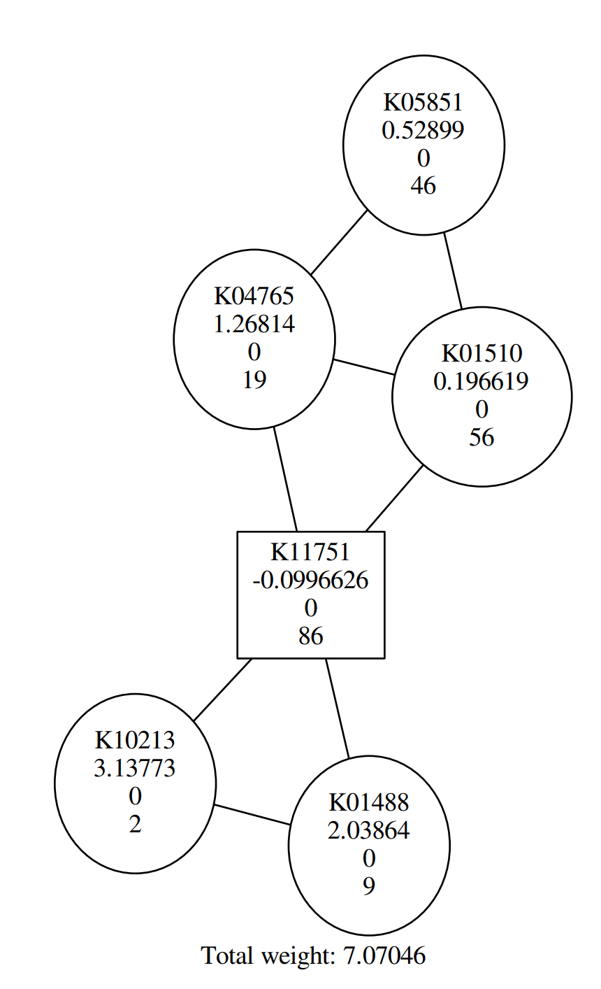
QuestionAccording to the figure above, Why are some shapes are round, others square?
Round shape corresponds to positive Heinz score; square shape corresponds to negative Heinz score.
In addition to the tool we will use in Galaxy, you may consider using eXamine plugin in Cytoscape for a richer visualization, if we use the original data from the study May et al., perform all of these steps and visualize the result by eXamine, we can get a visualization as follows:
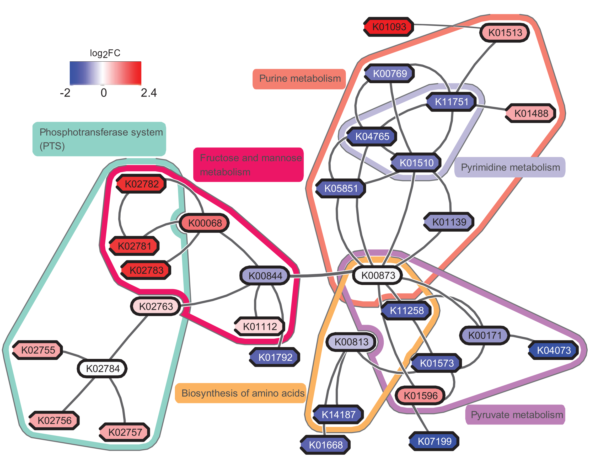
If you are interested, you may try to make sense of the result yourself. To answer the question “which pathways are potentially contributing to dental caries?”, we need to find the key pathways relevant to the subnetwork. To achieve that, we probably need to combine information from other bioinformatics services and literature.
Save the history into a workflow
Let’s assume that these are the operations we always need for different datasets, to make life easier, we can save all of these operations into a workflow in Galaxy, which you can reuse for different datasets next time.
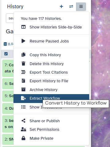
Hands On: Extract the Heinz workflow
Extract the workflow from your history
Clean up your history: remove any failed (red) jobs from your history by clicking on the galaxy-delete button.
This will make the creation of the workflow easier.
Click on galaxy-gear (History options) at the top of your history panel and select Extract workflow.
The central panel will show the content of the history in reverse order (oldest on top), and you will be able to choose which steps to include in the workflow.
Replace the Workflow name to something more descriptive.
Rename each workflow input in the boxes at the top of the second column.
If there are any steps that shouldn’t be included in the workflow, you can uncheck them in the first column of boxes.
Click on the Create Workflow button near the top.
You will get a message that the workflow was created.
Run the workflow on the dataset in this tutorial
As a self practice, you ran the newly created workflow with the dataset in this tutorial. Do you feel the convenience of running a workflow directly?
Congrats! You have finished all the tools in Heinz workflow! You have successfully run each tool and understood how it works. In real research, running these tools are only part of the effort, we still need to invest a huge amount of intelligence in making sense of the results and converting them to knowledge, which is fraught with uncertainties and confounders, where perhaps luck will come into play. So good luck!
You've Finished the Tutorial
Key points
Using Heinz do the network analysis based on the metatranscriptomics or transcriptomics data.
Extracting the signals hidden in the p-value distribution of the differential expression analysis.
Visualizing the pinpointed subnetwork helps us understand the result better
Heinz helps narrow down the scope to find the key pathways
Multiple CPUs will accelerate the computation especially for the complex datasets
Frequently Asked Questions
Have questions about this tutorial? Have a look at the available FAQ pages and support channelsUseful literature
Further information, including links to documentation and original publications, regarding the tools, analysis techniques and the interpretation of results described in this tutorial can be found here.
Feedback
Did you use this material as an instructor? Feel free to give us feedback on how it went.
Did you use this material as a learner or student? Click the form below to leave feedback.

Citing this Tutorial
- Chao Zhang, Network analysis with Heinz (Galaxy Training Materials). https://training.galaxyproject.org/training-material/topics/transcriptomics/tutorials/network-analysis-with-heinz/tutorial.html Online; accessed TODAY
- Hiltemann, Saskia, Rasche, Helena et al., 2023 Galaxy Training: A Powerful Framework for Teaching! PLOS Computational Biology 10.1371/journal.pcbi.1010752
- Batut et al., 2018 Community-Driven Data Analysis Training for Biology Cell Systems 10.1016/j.cels.2018.05.012
Congratulations on successfully completing this tutorial!@misc{transcriptomics-network-analysis-with-heinz, author = "Chao Zhang", title = "Network analysis with Heinz (Galaxy Training Materials)", year = "", month = "", day = "", url = "\url{https://training.galaxyproject.org/training-material/topics/transcriptomics/tutorials/network-analysis-with-heinz/tutorial.html}", note = "[Online; accessed TODAY]" } @article{Hiltemann_2023, doi = {10.1371/journal.pcbi.1010752}, url = {https://doi.org/10.1371%2Fjournal.pcbi.1010752}, year = 2023, month = {jan}, publisher = {Public Library of Science ({PLoS})}, volume = {19}, number = {1}, pages = {e1010752}, author = {Saskia Hiltemann and Helena Rasche and Simon Gladman and Hans-Rudolf Hotz and Delphine Larivi{\`{e}}re and Daniel Blankenberg and Pratik D. Jagtap and Thomas Wollmann and Anthony Bretaudeau and Nadia Gou{\'{e}} and Timothy J. Griffin and Coline Royaux and Yvan Le Bras and Subina Mehta and Anna Syme and Frederik Coppens and Bert Droesbeke and Nicola Soranzo and Wendi Bacon and Fotis Psomopoulos and Crist{\'{o}}bal Gallardo-Alba and John Davis and Melanie Christine Föll and Matthias Fahrner and Maria A. Doyle and Beatriz Serrano-Solano and Anne Claire Fouilloux and Peter van Heusden and Wolfgang Maier and Dave Clements and Florian Heyl and Björn Grüning and B{\'{e}}r{\'{e}}nice Batut and}, editor = {Francis Ouellette}, title = {Galaxy Training: A powerful framework for teaching!}, journal = {PLoS Comput Biol} }
You can use Ephemeris's
shed-tools installcommand to install the tools used in this tutorial.shed-tools install [-g GALAXY] [-a API_KEY] -t <(curl https://training.galaxyproject.org/training-material/api/topics/transcriptomics/tutorials/network-analysis-with-heinz/tutorial.json | jq .admin_install_yaml -r)Alternatively you can copy and paste the following YAML
---
install_tool_dependencies: true
install_repository_dependencies: true
install_resolver_dependencies: true
tools:
- name: deseq2
  owner: iuc
  revisions: d9e5cadc7f0b
  tool_panel_section_label: RNA Analysis
  tool_shed_url: https://toolshed.g2.bx.psu.edu/
- name: heinz
  owner: iuc
  revisions: 2b80a2596064
  tool_panel_section_label: RNA Analysis
  tool_shed_url: https://toolshed.g2.bx.psu.edu/
- name: heinz
  owner: iuc
  revisions: 2b80a2596064
  tool_panel_section_label: RNA Analysis
  tool_shed_url: https://toolshed.g2.bx.psu.edu/
- name: heinz
  owner: iuc
  revisions: 2b80a2596064
  tool_panel_section_label: RNA Analysis
  tool_shed_url: https://toolshed.g2.bx.psu.edu/
- name: heinz
  owner: iuc
  revisions: 5f589c91566e
  tool_panel_section_label: RNA Analysis
  tool_shed_url: https://toolshed.g2.bx.psu.edu/