Deep Learning (Part 3) - Convolutional neural networks (CNN)
| Author(s) |
|
| Reviewers |
|
OverviewQuestions:
Objectives:
What is a convolutional neural network (CNN)?
What are some applications of CNN?
Requirements:
Understand the inspiration behind CNN and learn the CNN architecture
Learn the convolution operation and its parameters
Learn how to create a CNN using Galaxy’s deep learning tools
Solve an image classification problem on MNIST digit classification dataset using CNN in Galaxy
- tutorial Hands-on: Introduction to deep learning
- slides Slides: Deep Learning (Part 1) - Feedforward neural networks (FNN)
- tutorial Hands-on: Deep Learning (Part 1) - Feedforward neural networks (FNN)
- slides Slides: Deep Learning (Part 2) - Recurrent neural networks (RNN)
- tutorial Hands-on: Deep Learning (Part 2) - Recurrent neural networks (RNN)
Time estimation: 2 hoursSupporting Materials:Published: Apr 19, 2021Last modification: May 11, 2026License: Tutorial Content is licensed under Creative Commons Attribution 4.0 International License. The GTN Framework is licensed under MITpurl PURL: https://gxy.io/GTN:T00257rating Rating: 4.0 (1 recent ratings, 8 all time)version Revision: 20
Artificial neural networks are a machine learning discipline that have been successfully applied to problems in pattern classification, clustering, regression, association, time series prediction, optimiztion, and control Jain et al. 1996. With the increasing popularity of social media in the past decade, image and video processing tasks have become very important. The previous neural network architectures (e.g. feedforward neural networks) could not scale up to handle image and video processing tasks. This gave way to the development of convolutional neural networks that are specifically tailored to image and video processing tasks. In this tutorial, we explain what convolutional neural networks are, discuss their architecture, and solve an image classification problem using MNIST digit classification dataset using a CNN in Galaxy.
AgendaIn this tutorial, we will cover:
Limitations of feedforward neural networks (FNN) for image processing
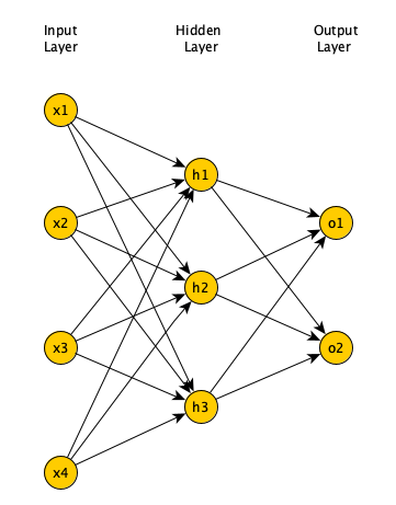
In a fully connected FNN (Figure 1), all the nodes in a layer are connected to all the nodes in the next layer. Each connection has a weight \(w\_{i,j}\) that needs to be learned by the learning algorithm. Lets say our input is a 64 pixel by 64 pixel grayscale image. Each grayscale pixel is represented by 1 value, usually between 0 to 255, where 0 represents black, 255 represents white, and the values in between represent various shades of gray. Since each grayscale pixel can be represented by 1 value, we say the channel size is 1. Such an image can be represented by 64 X 64 X 1 = 4,096 values (rows X columns X channels). Hence, the input layer of a FNN processing such an image has 4096 nodes.
Lets assume the next layer has 500 nodes. Since all the nodes in subsequent layers are fully connected, we will have 4,096 X 500 = 2,048,000 weights between the input and the first hidden layer. For complex problems, we usually need multiple hidden layers in our FNN, as a simpler FNN may not be able to learn the model mapping the inputs to outputs in the training data. Having multiple hidden layers compounds the problem of having many weights in our FNN. Having many weights makes the learning process more difficult as the dimension of the search space is increased. It also makes the training more time and resource consuming and increases the likelihood of overfitting. This problem is further compunded for color images. Unlike grayscale images, each pixel in a color image is represented by 3 values, representing red, green, and blue colors (Called RGB color mode), where every color can be represented by various combination of these primary colors. Since each color pixel can be represented by 3 values, we say the channel size is 3. Such an image can be represented by 64 X 64 X 3 = 12,288 values (rows X columns X channels). The number of weights between the input layer and the first hidden layer with 500 nodes is now 12,288 X 500 = 6,144,000. It is clear that a FNN cannot scale to handle larger images (O’Shea and Nash 2015) and that we need a more scalable architecture.
 Open image in new tab
Another problem with using FNN for image processing is that a 2 dimensional image is represented as a 1 dimensional vector in the input layer, hence, any spatial relationship in the data is ignored. CNN, on the other hand, maintains the spatial structure of the data, and is better suited for finding spatial relationships in the image data.
Inspiration for convolutional neural networks
In 1959 Hubel and Wiesel conducted an experiment to understand how the visual cortex of the brain processes visual information (Hubel and Wiesel 1959). They recorded the activity of the neurons in the visual cortex of a cat while moving a bright line in front of the cat. They noticed that some cells fire when the bright line is shown at a particular angle and a particular location (They called these simple cells). Other neurons fired when the bright line was shown regardless of the angle/location and seemed to detect movement (They called these complex cells). It seemed complex cells receive inputs from multiple simple cells and have an hierarchical structure. Hubel and Wiesel won the Noble prize for their findings in 1981.
In 1980, inspired by hierarchical structure of complex and simple cells, Fukushima proposed Neocognitron (Fukushima 1988), a hierarchical neural network used for handwritten Japanese character recognition. Neocognitron was the first CNN, and had its own training algorithm. In 1989, LeCun et. al. (LeCun et al. 1989) proposed a CNN that could be trained by backpropagation algorithm. CNN gained immense popularity when they outperformed other models at ILSVRC (ImageNet Large Scale Visual Recognition Challenge). ILSVRC is a competition in object classification and detection on hundreds of object categories and millions of images. The challenge has been run annually from 2010 to present, attracting participation from more than fifty institutions (Russakovsky et al. 2015). Notable CNN architectures that won ILSVRC are AlexNet in 2012 (Krizhevsky et al. 2012), ZFNet in 2013 ( Zeiler and Fergus 2013), GoogLeNet and VGG in 2014 (Szegedy et al. 2014, Simonyan and Zisserman 2015), and ResNet in 2015 (He et al. 2015).
Architecture of CNN
A typical CNN has the following 4 layers (O’Shea and Nash 2015)
- Input layer
- Convolution layer
- Pooling layer
- Fully connected layer
Please note that we will explain a 2 dimensional (2D) CNN here. But the same concepts apply to a 1 (or 3) dimensional CNN as well.
Input layer
The input layer represents the input to the CNN. An example input, could be a 28 pixel by 28 pixel grayscale image. Unlike FNN, we do not “flatten” the input to a 1D vector, and the input is presented to the network in 2D as a 28 x 28 matrix. This makes capturing spatial relationships easier.
Convolution layer
The convolution layer is composed of multiple filters (also called kernels). Filters for a 2D image are also 2D. Suppose we have a 28 pixel by 28 pixel grayscale image. Each pixel is represented by a number between 0 and 255, where 0 represents the color black, 255 represents the color white, and the values in between represent different shades of gray. Suppose we have a 3 by 3 filter (9 values in total), and the values are randomly set to 0 or 1. Convolution is the process of placing the 3 by 3 filter on the top left corner of the image, multiplying filter values by the pixel values and adding the results, moving the filter to the right one pixel at a time and repeating this process. When we get to the top right corner of the image, we simply move the filter down one pixel and restart from the left. This process ends when we get to the bottom right corner of the image.
 Open image in new tab
Covolution operator has the following parameters:
- Filter size
- Padding
- Stride
- Dilation
- Activation function
Filter size can be 5 by 5, 3 by 3, and so on. Larger filter sizes should be avoided as the learning algorithm needs to learn filter values (weights), and larger filters increase the number of weights to be learned (more compute capacity, more training time, more chance of overfitting). Also, odd sized filters are preferred to even sized filters, due to the nice geometric property of all the input pixels being around the output pixel.
If you look at Figure 2 you see that after applying a 3 by 3 filter to a 4 by 4 image, we end up with a 2 by 2 image – the size of the image has gone down. If we want to keep the resultant image size the same, we can use padding. We pad the input in every direction with 0’s before applying the filter. If the padding is 1 by 1, then we add 1 zero in evey direction. If its 2 by 2, then we add 2 zeros in every direction, and so on.
 Open image in new tab
As mentioned before, we start the convolution by placing the filter on the top left corner of the image, and after multiplying filter and image values (and adding them), we move the filter to the right and repeat the process. How many pixels we move to the right (or down) is the stride. In figure 2 and 3, the stride of the filter is 1. We move the filter one pixel to the right (or down). But we could use a different stride. Figure 4 shows an example of using stride of 2.
 Open image in new tab
When we apply a, say 3 by 3, filter to an image, our filter’s output is affected by pixels in a 3 by 3 subset of the image. If we like to have a larger receptive field (portion of the image that affect our filter’s output), we could use dilation. If we set the dilation to 2 (Figure 5), instead of a contiguous 3 by 3 subset of the image, every other pixel of a 5 by 5 subset of the image affects the filter’s output.
 Open image in new tab
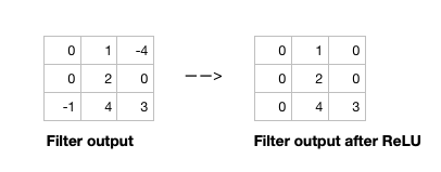
After the filter scans the whole image, we apply an activation function to filter output to introduce non-linearlity. The preferred activation function used in CNN is ReLU or one its variants like Leaky ReLU (Nwankpa et al. 2018). ReLU leaves pixels with positive values in filter output as is, and replacing negative values with 0 (or a small number in case of Leaky ReLU). Figure 6 shows the results of applying ReLU activation function to a filter output.
 Open image in new tab
Given the input size, filter size, padding, stride and dilation you can calculate the output size of the convolution operation as below.
\[\frac{(\text{input size} - \text{(filter size + (filter size -1)*(dilation - 1)})) + (2*padding)}{stride} + 1\]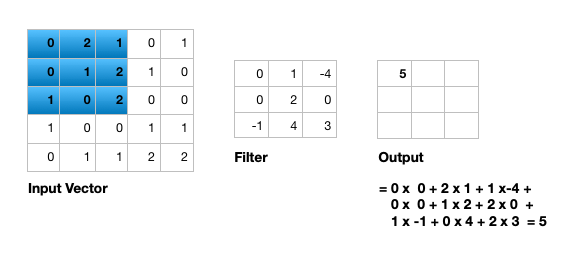 Open image in new tab
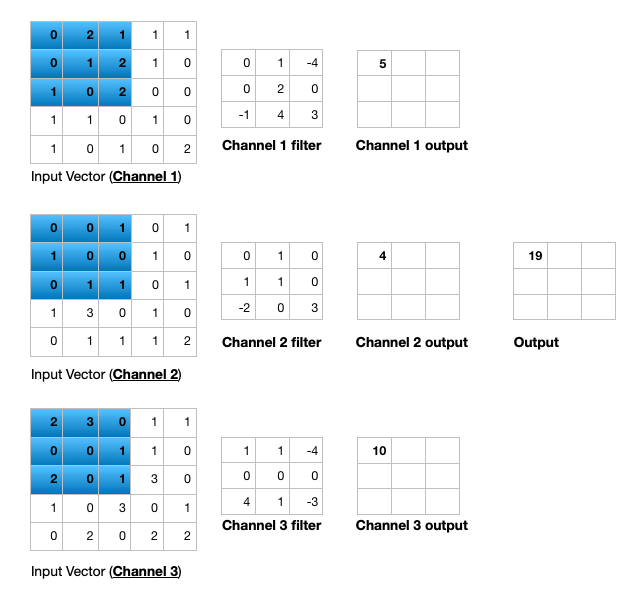
Figure 7 illustrates the calculations for a convolution operation, via a 3 by 3 filter on a single channel 5 by 5 input vector (5 x 5 x 1). Figure 8 illustrates the calculations when the input vector has 3 channels (5 x 5 x 3). To show this in 2 dimensions, we are displaying each channel in input vector and filter separately. Figure 9 shows a sample multi-channel 2D convolution in 3 dimensions.
 Open image in new tab
As Figures 8 and 9 show the output of a multi-channel 2 dimensional filter is a single channel 2 dimensional image. Applying multiple filters to the input image results in a multi-channel 2 dimensional image for the output. For example, if the input image is 28 by 28 by 3 (rows x columns x channels), and we apply a 3 by 3 filter with 1 by 1 padding, we would get a 28 by 28 by 1 image. If we apply 15 filters to the input image, our output would be 28 by 28 by 15. Hence, the number of filters in a convolution layer allows us to increase or decrease the channel size.
 Open image in new tab
Pooling layer
The pooling layer performs down sampling to reduce the spatial dimensionality of the input. This decreases the number of parameters, which in turn reduces the learning time and computation, and the likelihood of overfitting. The most popular type of pooling is max pooling. Its usually a 2 by 2 filter with a stride of 2 that returns the maximum value as it slides over the input data (similar to convolution filters).
Fully connected layer
The last layer in a CNN is a fully connected layer. We connect all the nodes from the previous layer to this fully connected layer, which is responsible for classification of the image.
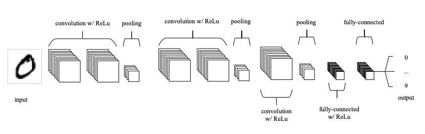 Open image in new tab
As shown in Figure 10, a typical CNN usually has more than one convolution layer plus pooling layer. Each convolution plus pooling layer is responsible for feature extraction at a different level of abstraction. For example, the filters in the first layer could detect horizental, vertical, and diagonal edges. The filters in the next layer could detect shapes, and the filters in the last layer could detect collection of shapes. Filter values are randomly initialized and are learned by the learning algorithm. This makes CNN very powerful as they not only do classification, but can also automatically do feature extraction. This distinguishes CNN from other classification techniques (like Support Vector Machines), which cannot do feature extraction.
MNIST dataset
The MNIST database of handwritten digits (LeCun et al. 2010) is composed of a training set of 60,000 images and a test set of 10,000 images. The digits have been size-normalized and centered in a fixed-size image (28 by 28 pixels). Images are grayscale, where each pixel is represented by a number between 0 and 255 (0 for black, 255 for white, and other values for different shades of gray). MNIST database is a standard image classification dataset and is used to compare various Machine Learning techniques.
Get data
Hands On: Data upload
Make sure you have an empty analysis history.
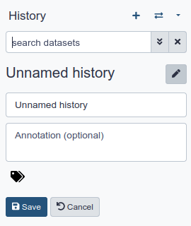
To create a new history simply click the new-history icon at the top of the history panel:
Rename your history to make it easy to recognize
Click on the title of the history (by default the title is
Unnamed history)
- Type
Galaxy Introductionas the name- Press Enter
Import the files from Zenodo
https://zenodo.org/record/4697906/files/X_train.tsv
https://zenodo.org/record/4697906/files/y_train.tsv
https://zenodo.org/record/4697906/files/X_test.tsv
https://zenodo.org/record/4697906/files/y_test.tsv
- Copy the link location
Click galaxy-upload Upload at the top of the activity panel
- Select galaxy-wf-edit Paste/Fetch Data
Paste the link(s) into the text field
Press Start
- Close the window
Rename the datasets as
X_train,y_train,X_test, andy_testrespectively.
- Click on the galaxy-pencil pencil icon for the dataset to edit its attributes
- In the central panel, change the Name field
- Click the Save button
Check that the datatype of all four datasets is
tabular.
- Click on the galaxy-pencil pencil icon for the dataset to edit its attributes
- In the central panel, click galaxy-chart-select-data Datatypes tab on the top
- In the galaxy-chart-select-data Assign Datatype, select
datatypesfrom “New Type” dropdown
- Tip: you can start typing the datatype into the field to filter the dropdown menu
- Click the Save button


Classification of MNIST dataset images with CNN
In this section, we define a CNN and train it using MNIST dataset training data. The goal is to learn a model such that given an image of a digit we can predict whether the digit (0 to 9). We then evaluate the trained CNN on the test dataset and plot the confusion matrix.
In order to train the CNN, we must have the One-Hot Encoding (OHE) representation of the training labels. This is needed to calculate the categorical cross entropy loss function. OHE encodes labels as a one-hot numeric array, where only one element is 1 and the rest are 0’s. For example, if we had 3 fruits (apple, orange, banana) and their labels were 1, 2, and 3, the OHE represntation of apple would be (1,0,0), the OHE representation of orange would be (0,1,0), and the OHE representation of banana would be (0,0,1). For apple with label 1, the first element of array is 1 (and the rest are 0’s); For Orange with label 2, the second element of the array is 1 (and the rest are 0’s); And for Banana with label 3, the third element of the array is 1 (and the rest are 0’s). We have 10 digits in our dataset and we would just have an array of size 10, where only one element is 1, corresponding to the digit, and the rest are 0’s.
Create One-Hot Encoding (OHE) representation of training labels
Hands On: One-Hot Encoding
- To categorical ( Galaxy version 1.0.10.0)
- “Total number of classes”: Select
10- “Input file” : Select
y_train- “Does the dataset contain header?” : Select
No- Click “Run Tool”
Create a deep learning model architecture
Hands On: Model config
- Create a deep learning model architecture ( Galaxy version 1.0.10.0)
- “Select keras model type”:
sequential- “input_shape”:
(784,)- In “LAYER”:
- param-repeat “1: LAYER”:
- “Choose the type of layer”:
Core -- Reshape
- “target_shape”:
(28,28,1)- param-repeat “2: LAYER”:
- “Choose the type of layer”:
Convolutional -- Conv2D
- “filters”:
64- “kernel_size”:
3- “Activation function”:
relu- “Type in key words arguments if different from the default”:
padding='same'- param-repeat “3: LAYER”:
- “Choose the type of layer”:
Pooling -- MaxPooling2D
- “pool_size”:
(2,2)- param-repeat “4: LAYER”:
- “Choose the type of layer”:
Convolutional -- Conv2D
- “filters”:
32- “kernel_size”:
3- “Activation function”:
relu- param-repeat “5: LAYER”:
- “Choose the type of layer”:
Pooling -- MaxPooling2D
- “pool_size”:
(2,2)- param-repeat “6: LAYER”:
- “Choose the type of layer”:
Core -- Flatten- param-repeat “7: LAYER”:
- “Choose the type of layer”:
Core -- Dense
- “units””:
10- “Activation function”:
softmax- Click “Run Tool”
Each image is passed in as a 784 dimensional vector (28 x 28 = 784). The reshape layer reshapes it into (28, 28, 1) dimensions – 28 rows (image height), 28 columns (image width), and 1 channel. Channel is 1 since the image is grayscale and each pixel can be represented by one integer. Color images are represented by 3 integers (RGB values) and have channel size 3. Our CNN then has 2 convolution + pooling layers. First convolution layer has 64 filters (output would be 64 dimensional), and filter size is 3 x 3. Second convolutional layer has 32 filters (output would be 32 dimensional), and filter size is 3 x 3. Both pooling layers are MaxPool layers with pool size of 2 by 2. Afterwards, we flatten the previous layers output (every row/colum/channel would be an individual node). Finally, we add a fully connected layer with 10 nodes and use a softmax activation function to get the probability of each digit. Digit with the highest probability is predicted by CNN. The model config can be downloaded as a JSON file.
Create a deep learning model
Hands On: Model builder (Optimizer, loss function, and fit parameters)
- Create deep learning model ( Galaxy version 1.0.10.0)
- “Choose a building mode”:
Build a training model- “Select the dataset containing model configuration”: Select the Keras Model Config from the previous step.
- “Do classification or regression?”:
KerasGClassifier- In “Compile Parameters”:
- “Select a loss function”:
categorical_crossentropy- “Select an optimizer”:
Adam - Adam optimizer- “Select metrics”:
acc/accuracy- In “Fit Parameters”:
- “epochs”:
2- “batch_size”:
500- Click “Run Tool”
A loss function measures how different the predicted output is versus the expected output. For multi-class classification problems, we use categorical cross entropy as loss function. Epochs is the number of times the whole training data is used to train the model. Setting epochs to 2 means each training example in our dataset is used twice to train our model. If we update network weights/biases after all the training data is feed to the network, the training will be very slow (as we have 60000 training examples in our dataset). To speed up the training, we present only a subset of the training examples to the network, after which we update the weights/biases. The batch_size decides the size of this subset. The model builder can be downloaded as a zip file.
Deep learning training and evaluation
Hands On: Training the model
- Deep learning training and evaluation ( Galaxy version 1.0.11.0)
- “Select a scheme”:
Train and Validate- “Choose the dataset containing pipeline/estimator object”: Select the Keras Model Builder from the previous step.
- “Select input type:”:
tabular data
- “Training samples dataset”: Select
X_traindataset- “Choose how to select data by column:”:
All columns- “Dataset containing class labels or target values”:
To categorical on y_train(the output of the first step)- “Choose how to select data by column:”:
All columns- Click “Run Tool”
The training step generates 3 datasets: 1) accuracy of the trained model, 2) the trained model architecture file, downloadable as a tabular file, and 3) the trained model weights, downloadable as an hdf5 (or h5mlm) file. These files are needed for prediction in the next step.
Model Prediction
Hands On: Testing the model
- Model Prediction ( Galaxy version 1.0.11.0)
- “Choose the dataset containing pipeline/estimator object” : Select the trained model from the previous step.
- “Select invocation method”:
predict- “Select input data type for prediction”:
tabular data- “Training samples dataset”: Select
X_testdataset- “Choose how to select data by column:”:
All columns- Click “Run Tool”
The prediction step generates 1 dataset. It’s a file that has predictions (0 to 9 for the predicted digits) for every image in the test dataset.
Machine Learning Visualization Extension
Hands On: Creating the confusion matrix
- Machine Learning Visualization Extension ( Galaxy version 1.0.11.0)
- “Select a plotting type”:
Confusion matrix for classes- “Select dataset containing the true labels””:
y_test- “Choose how to select data by column:”:
All columns- “Select dataset containing the predicted labels””: Select
Model Predictionfrom the previous step- “Does the dataset contain header:”:
Yes- Click “Run Tool”
Confusion Matrix is a table that describes the performance of a classification model. It lists the number of examples that were correctly classified by the model, True positives (TP) and true negatives (TN). It also lists the number of examples that were classified as positive that were actually negative (False positive, FP, or Type I error), and the number of examples that were classified as negative that were actually positive (False negative, FN, or Type 2 error). Given the confusion matrix, we can calculate precision and recall Tatbul et al. 2018. Precision is the fraction of predicted positives that are true positives (Precision = TP / (TP + FP)). Recall is the fraction of true positives that are predicted (Recall = TP / (TP + FN)). One way to describe the confusion matrix with just one value is to use the F score, which is the harmonic mean of precision and recall
\[Precision = \frac{\text{True positives}}{\text{True positives + False positives}}\] \[Recall = \frac{\text{True positives}}{\text{True positives + False negatives}}\] \[F score = \frac{2 * \text{Precision * Recall}}{\text{Precision + Recall}}\]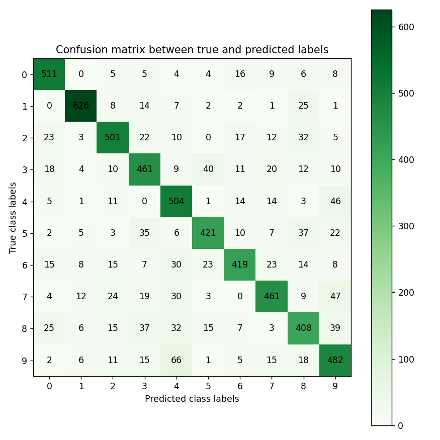 Open image in new tab
Figure 11 is the resultant confusion matrix for our image problem. The first row in the table represents the true digit 0 class labels (we have 541 + 1 + 2 + 1 + 1 + 5 + 9 + 1 + 3 + 4 = 568 digit 0 images). The second row represents the true digit 1 class labels (Again, we have 665 + 5 + 5 + 3 + 2 + 2 + 4 = 686 digit 1 images). Similarly, you can count the true class labels for digits 2 to 9 by adding up the numbers in the coresponding row. The first column from the left represents the predicted digit 0 class labels (Our CNN predicted 541 + 1 + 3 + 2 + 7 + 1 + 15 = 570 images as being digit 0). The second column from the left represents the predicted digit 1 class labels (Our CNN predicted 665 + 1 + 4 + 2 + 7 + 5 + 1 + 4 = 689 images as being digit 1). Similarly, you can count the predicted class labels for digits 2 to 9 by adding up the numbers in the corresponding column.
For digit 0, looking at the top-left green cell, we see that our CNN has correctly predicted 541 images as digit 0 (True positives). Adding the numbers in the left most column besides the True positives (1 + 3 + 2 + 7 + 1 + 15 = 29), we see that our CNN has incorrectly predicted 29 images as being digit 0 (False positives). Adding the numbers on the top row besides the True positives (1 + 2 + 1 + 1 + 5 + 9 + 1 + 3 + 4 = 27), we see that our CNN has incorrectly predicted 27 digits 0 images as not being digit 0 (False negatives). Given these numbers we can calculate Precision, Recall, and the F score for digit 0 as follows:
\[Precision = \frac{\text{True positives}}{\text{True positives + False positives}} = \frac{541}{541 + 29} = 0.949\] \[Recall = \frac{\text{True positives}}{\text{True positives + False negatives}} = \frac{541}{541 + 27} = 0.952\] \[F score = \frac{2 * \text{Precision * Recall}}{\text{Precision + Recall}} = \frac{2 * 0.949 * 0.952}{0.949 + 0.952} = 0.950\]You can calculate the Precision, Recall, and F score for other digits in a similar manner.
Conclusion
In this tutorial, we explained the motivation for convolutional neural networks, explained their architecture, and discussed convolution operator and its parameters. We then used Galaxy to solve an image classification problem using CNN on MNIST dataset.
You've Finished the Tutorial
Frequently Asked Questions
Have questions about this tutorial? Have a look at the available FAQ pages and support channelsReferences
- Hubel, D. H., and T. N. Wiesel, 1959 Receptive fields of single neurones in the cat’s striate cortex. The Journal of physiology 148: 574–591. 10.1113/jphysiol.1959.sp006308
- Fukushima, K., 1988 Neocognitron: A hierarchical neural network capable of visual pattern recognition. Neural Networks 1: 119–130. https://doi.org/10.1016/0893-6080(88)90014-7 https://www.sciencedirect.com/science/article/pii/0893608088900147
- LeCun, Y., B. Boser, J. S. Denker, D. Henderson, R. E. Howard et al., 1989 Backpropagation Applied to Handwritten Zip Code Recognition. Neural Computation 1: 541–551. 10.1162/neco.1989.1.4.541
- Jain, A. K., J. Mao, and K. M. Mohiuddin, 1996 Artificial neural networks: a tutorial. Computer 29: 31–44. 10.1109/2.485891
- LeCun, Y., C. Cortes, and C. J. Burges, 2010 MNIST handwritten digit database. ATT Labs [Online]. Available: http://yann.lecun.com/exdb/mnist 2:
- Krizhevsky, A., I. Sutskever, and G. Hinton, 2012 ImageNet Classification with Deep Convolutional Neural Networks. Neural Information Processing Systems 25: 10.1145/3065386
- Zeiler, M. D., and R. Fergus, 2013 Visualizing and Understanding Convolutional Networks. ECCV. 1311.2901
- Szegedy, C., W. Liu, Y. Jia, P. Sermanet, S. Reed et al., 2014 Going Deeper with Convolutions. CVPR. 1409.4842
- He, K., X. Zhang, S. Ren, and J. Sun, 2015 Deep Residual Learning for Image Recognition. CVPR. 1512.03385
- O’Shea, K., and R. Nash, 2015 An Introduction to Convolutional Neural Networks. CoRR abs/1511.08458: http://arxiv.org/abs/1511.08458
- Russakovsky, O., J. Deng, H. Su, J. Krause, S. Satheesh et al., 2015 ImageNet Large Scale Visual Recognition Challenge. International Journal of Computer Vision 115: 2211–252. 10.1007/s11263-015-0816-y
- Simonyan, K., and A. Zisserman, 2015 Very Deep Convolutional Networks for Large-Scale Image Recognition. CVPR. 1409.1556
- Dumoulin, V., and F. Visin, 2016 A guide to convolution arithmetic for deep learning. 1603.07285
- Nwankpa, C., W. Ijomah, A. Gachagan, and S. Marshall, 2018 Activation Functions: Comparison of trends in Practice and Research for Deep Learning. CoRR abs/1811.03378: http://arxiv.org/abs/1811.03378
- Tatbul, N., T. J. Lee, S. Zdonik, M. Alam, and J. Gottschlich, 2018 Precision and Recall for Time Series. Advances in Neural Information Processing Systems 31: 1920–1930. https://proceedings.neurips.cc/paper/2018/file/8f468c873a32bb0619eaeb2050ba45d1-Paper.pdf
Feedback
Did you use this material as an instructor? Feel free to give us feedback on how it went.
Did you use this material as a learner or student? Click the form below to leave feedback.

Citing this Tutorial
- Kaivan Kamali, Deep Learning (Part 3) - Convolutional neural networks (CNN) (Galaxy Training Materials). https://training.galaxyproject.org/training-material/topics/statistics/tutorials/CNN/tutorial.html Online; accessed TODAY
- Hiltemann, Saskia, Rasche, Helena et al., 2023 Galaxy Training: A Powerful Framework for Teaching! PLOS Computational Biology 10.1371/journal.pcbi.1010752
- Batut et al., 2018 Community-Driven Data Analysis Training for Biology Cell Systems 10.1016/j.cels.2018.05.012
Congratulations on successfully completing this tutorial!@misc{statistics-CNN, author = "Kaivan Kamali", title = "Deep Learning (Part 3) - Convolutional neural networks (CNN) (Galaxy Training Materials)", year = "", month = "", day = "", url = "\url{https://training.galaxyproject.org/training-material/topics/statistics/tutorials/CNN/tutorial.html}", note = "[Online; accessed TODAY]" } @article{Hiltemann_2023, doi = {10.1371/journal.pcbi.1010752}, url = {https://doi.org/10.1371%2Fjournal.pcbi.1010752}, year = 2023, month = {jan}, publisher = {Public Library of Science ({PLoS})}, volume = {19}, number = {1}, pages = {e1010752}, author = {Saskia Hiltemann and Helena Rasche and Simon Gladman and Hans-Rudolf Hotz and Delphine Larivi{\`{e}}re and Daniel Blankenberg and Pratik D. Jagtap and Thomas Wollmann and Anthony Bretaudeau and Nadia Gou{\'{e}} and Timothy J. Griffin and Coline Royaux and Yvan Le Bras and Subina Mehta and Anna Syme and Frederik Coppens and Bert Droesbeke and Nicola Soranzo and Wendi Bacon and Fotis Psomopoulos and Crist{\'{o}}bal Gallardo-Alba and John Davis and Melanie Christine Föll and Matthias Fahrner and Maria A. Doyle and Beatriz Serrano-Solano and Anne Claire Fouilloux and Peter van Heusden and Wolfgang Maier and Dave Clements and Florian Heyl and Björn Grüning and B{\'{e}}r{\'{e}}nice Batut and}, editor = {Francis Ouellette}, title = {Galaxy Training: A powerful framework for teaching!}, journal = {PLoS Comput Biol} }
You can use Ephemeris's
shed-tools installcommand to install the tools used in this tutorial.shed-tools install [-g GALAXY] [-a API_KEY] -t <(curl https://training.galaxyproject.org/training-material/api/topics/statistics/tutorials/CNN/tutorial.json | jq .admin_install_yaml -r)Alternatively you can copy and paste the following YAML
---
install_tool_dependencies: true
install_repository_dependencies: true
install_resolver_dependencies: true
tools:
- name: keras_model_builder
  owner: bgruening
  revisions: 66d7efc06000
  tool_panel_section_label: Machine Learning
  tool_shed_url: https://toolshed.g2.bx.psu.edu/
- name: keras_model_config
  owner: bgruening
  revisions: f22a9297440f
  tool_panel_section_label: Machine Learning
  tool_shed_url: https://toolshed.g2.bx.psu.edu/
- name: keras_train_and_eval
  owner: bgruening
  revisions: aeee74692508
  tool_panel_section_label: Machine Learning
  tool_shed_url: https://toolshed.g2.bx.psu.edu/
- name: ml_visualization_ex
  owner: bgruening
  revisions: 5f9c0e99016f
  tool_panel_section_label: Machine Learning
  tool_shed_url: https://toolshed.g2.bx.psu.edu/
- name: model_prediction
  owner: bgruening
  revisions: 475b5171945f
  tool_panel_section_label: Machine Learning
  tool_shed_url: https://toolshed.g2.bx.psu.edu/
- name: sklearn_to_categorical
  owner: bgruening
  revisions: 61634a87efc7
  tool_panel_section_label: Machine Learning
  tool_shed_url: https://toolshed.g2.bx.psu.edu/