After sequencing and assembly, a genome can be annotated. It is an essential step to describe the genome.

Genome annotation consists in describing the structure and function of the components of the genome, by predicting, analyzing, and interpreting them in order to extract their biological significance and understand the biological processes in which they participate. Among other things, it identifies the locations of genes and all the coding regions in a genome (structural annotation) and determines what those genes do (functional annotation).

To illustrate the process to annotate a bacterial genome, we take an assembly of a bacterial genome (KUN1163 sample) generated by following a bacterial genome assembly tutorial from data produced in “Complete Genome Sequences of Eight Methicillin-Resistant Staphylococcus aureus Strains Isolated from Patients in Japan” (Hikichi et al. 2019).

Methicillin-resistant Staphylococcus aureus (MRSA) is a major pathogen causing nosocomial infections, and the clinical manifestations of MRSA range from asymptomatic colonization of the nasal mucosa to soft tissue infection to fulminant invasive disease. Here, we report the complete genome sequences of eight MRSA strains isolated from patients in Japan.

Agenda

In this tutorial, we will cover:

1. Galaxy and data preparation
2. Contig annotation
3. Further structural annotation
   1. Plasmids
   2. Integrons
   3. IS (Insertion Sequence) elements
4. Visualisation of the annotation
5. Conclusion

Galaxy and data preparation

Any analysis should get its own Galaxy history. So let’s start by creating a new one and get the data (contig file from the assembly) into it.

Hands-on: Prepare Galaxy and data

1. Create a new history for this analysis

   Tip: Creating a new history

   Click the new-history icon at the top of the history panel:

   

2. Rename the history

   Tip: Renaming a history

   1. Click on galaxy-pencil (Edit) next to the history name (which by default is “Unnamed history”)
   2. Type the new name
   3. Click on Save

   If you do not have the galaxy-pencil (Edit) next to the history name:

   1. Click on Unnamed history (or the current name of the history) (Click to rename history) at the top of your history panel
   2. Type the new name
   3. Press Enter

3. Import the contig file from Zenodo or from Galaxy shared data libraries:

   https://zenodo.org/record/10572227/files/DRR187559_contigs.fasta
   

   Tip: Importing via links

   • Copy the link location

   • Click galaxy-upload Upload Data at the top of the tool panel

   • Select galaxy-wf-edit Paste/Fetch Data

   • Paste the link(s) into the text field

   • Press Start

   • Close the window

   Tip: Importing data from a data library

   As an alternative to uploading the data from a URL or your computer, the files may also have been made available from a shared data library:

   1. Go into Shared data (top panel) then Data libraries
   2. Navigate to the correct folder as indicated by your instructor.
      • On most Galaxies tutorial data will be provided in a folder named GTN - Material –> Topic Name -> Tutorial Name.
   3. Select the desired files
   4. Click on Add to History galaxy-dropdown near the top and select as Datasets from the dropdown menu

   5. In the pop-up window, choose

      • “Select history”: the history you want to import the data to (or create a new one)
   6. Click on Import

Contig annotation

For annotating the contigs, several tools exists to do that: Prokka (Seemann 2014), Bakta (Schwengers et al. 2021), etc. Here, we use Bakta as recommended by Torsten Seemann as the successor of Prokka.

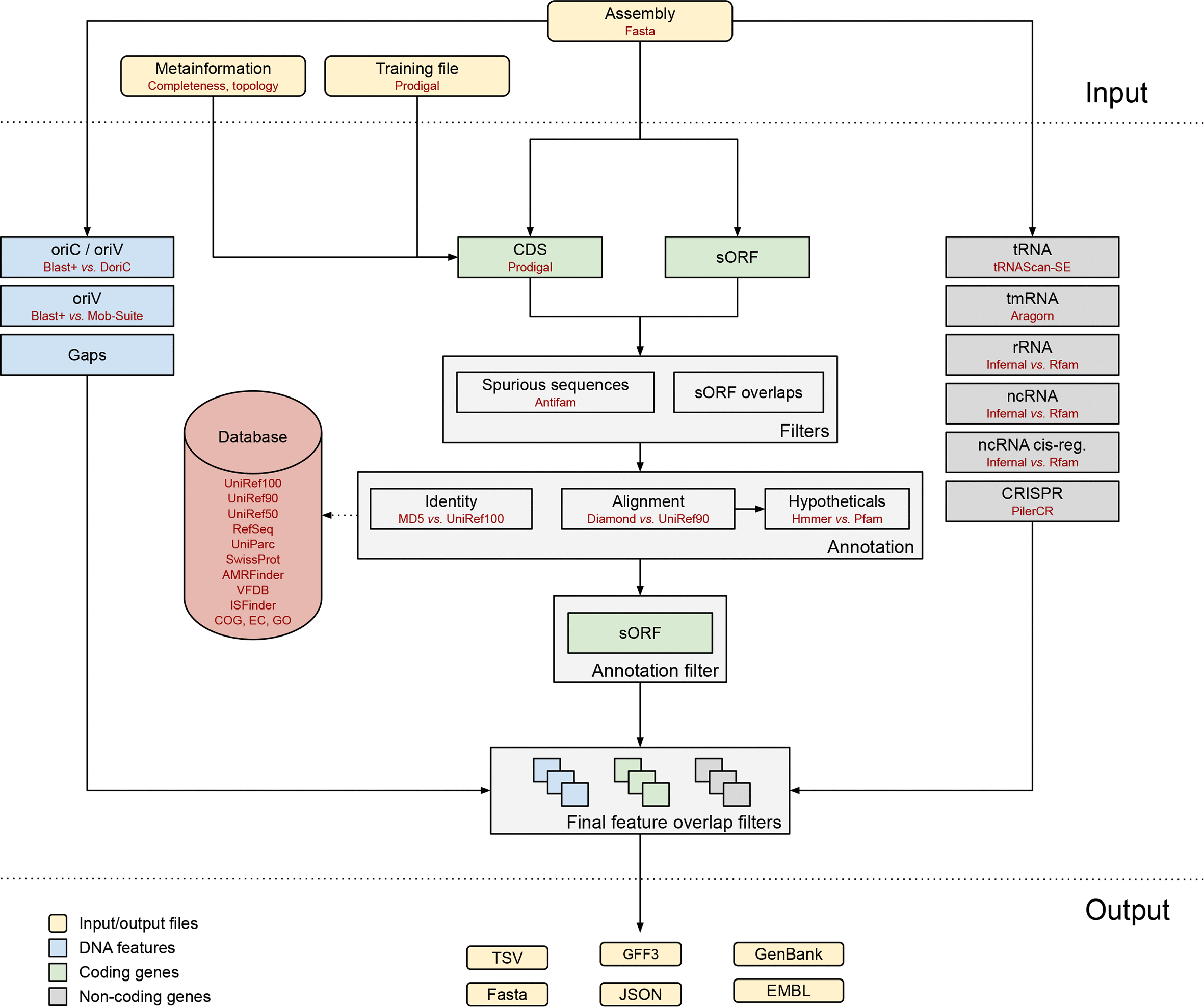
Bakta is a tool for the rapid & standardized annotation of bacterial genomes and plasmids from both isolates and metagenome-assembled genomes (MAGs). It implements a comprehensive annotation workflow for coding and non-coding genes (i.e. tRNA, rRNA).

Open image in new tab

It is also able to detect and annotate small proteins (sORF). Predicted CDS are annotated using an alignment-free protein sequence identification approach with cross-references to public databases via stable identifiers.

Hands-on: Contig annotation

1. Bakta ( Galaxy version 1.8.2+galaxy0) with the following parameters:
   • In “Input/Output options”:
     • “The bakta database”: latest one
     • “The amrfinderplus database”: latest one
     • param-file “Select genome in fasta format”: Contig file
   • In “Optional annotation”:
     • “Keep original contig header (–keep-contig-headers)”: Yes
   • In “Selection of the output files”:
     • “Output files selection”:
       • Annotation file in TSV
       • Annotation and sequence in GFF3
       • Feature nucleotide sequences as FASTA
       • Summary as TXT
       • Plot of the annotation result as SVG

Bakta can generate many outputs. Here we selected:

• Analysis_summary: a summary of the analysis as text file

  Question

  1. How many contigs have been provided as input?
  2. How long is the draft genome?
  3. How many CDSs have been found?
  4. How many small proteins?
  5. Which other components have been found?

  How does it compare to results for KUN1163 in Table 1 in Hikichi et al. 2019?

  Solution

  1. 44 (the sequence count)
  2. 2,911,349 bp, with is a bit shorter than the expected 2,914,567 bp in Table 1 in Hikichi et al. 2019
  3. 2,717 CDSs, a bit more than the expected 2,704 CDSs in Table 1 in Hikichi et al. 2019
  4. 5 sORFs. There is no information about sORFs in Hikichi et al. 2019

  5. Other components

     Components	Bakta	Hikichi et al. 2019
     tRNAs	57	61
     Transfer-messenger RNA (tmRNAs)	1	1
     rRNAs	9	5
     ncRNAs	95	No information

• Nucleotide_sequences with feature nucleotide sequences as FASTA file

  Question

  1. How many sequences are in this file?
  2. What are the sequences stored there?

  Solution

  1. 2,884 sequences
  2. Here are stored:
     • tRNAs
     • tmRNAs
     • rRNAs
     • ncRNAs
     • CDSs
     • sORFs

• annotation_summary with annotations as simple human readble TSV

  Question

  What is stored there?

  Solution

  This a table with 9 columns (Sequence Id, Type, Start, Stop, Strand, Locus Tag, Gene, Product, DbXrefs). It contains here 2,916 lines, so the information and location for:

  • tRNAs
  • tmRNAs
  • rRNAs
  • ncRNAs
  • CDSs
  • sORFs
  • gaps
  • oriCs
  • oriVs
  • oriTs

• Annotation_and_sequences in GFF3

  GFF is a file format used for describing genes and other features of DNA, RNA and protein sequences. It is a tab delimited file with 9 fields per line:

  1. seqid: The name of the sequence where the feature is located.
  2. source: The algorithm or procedure that generated the feature. This is typically the name of a software or database.
  3. type: The feature type name, like “gene” or “exon”. In a well structured GFF file, all the children features always follow their parents in a single block (so all exons of a transcript are put after their parent “transcript” feature line and before any other parent transcript line). In GFF3, all features and their relationships should be compatible with the standards released by the Sequence Ontology Project.
  4. start: Genomic start of the feature, with a 1-base offset. This is in contrast with other 0-offset half-open sequence formats, like BED.
  5. end: Genomic end of the feature, with a 1-base offset. This is the same end coordinate as it is in 0-offset half-open sequence formats, like BED.
  6. score: Numeric value that generally indicates the confidence of the source in the annotated feature. A value of “.” (a dot) is used to define a null value.
  7. strand: Single character that indicates the strand of the feature. This can be “+” (positive, or 5’->3’), “-“, (negative, or 3’->5’), “.” (undetermined), or “?” for features with relevant but unknown strands.
  8. phase: phase of CDS features; it can be either one of 0, 1, 2 (for CDS features) or “.” (for everything else). See the section below for a detailed explanation.
  9. attributes: A list of tag-value pairs separated by a semicolon with additional information about the feature.

  Question

  How many features are annotated?

  Solution

  51k+ (number of lines in the GFF)

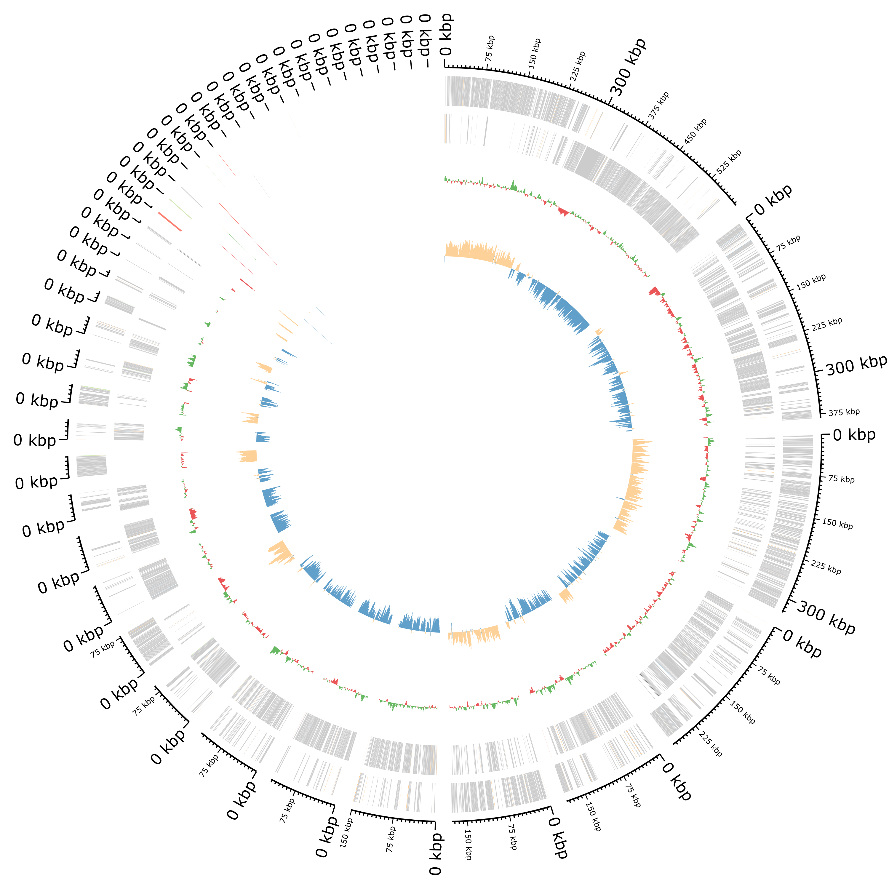
• Plot of the annotation as circular genome annotation

  

  Question

  1. What the 2 rings in the center?
  2. How are plotted the features?

  Solution

  1. The first ring represents the GC content per sliding window over the entire sequence(s) with in green representing GC above and red GC below average. The 2nd ring represents the GC skew in orange and blue.
  2. All features are plotted on two rings representing the forward and reverse strand from outer to inner with CDS in grey (the other colors are hard to distinguish)

Further structural annotation

Bakta gives a lot of information already, especially regarding CDSs or RNAs, but some structural annotation might be missing, e.g. plasmids, or interesting to identify independently.

Plasmids

To identify plasmids in our contigs, we use PlasmidFinder (Carattoli and Hasman 2020), a tool for the identification and typing of plasmid sequences in Whole-Genome Sequencing. It uses the plasmidfinder database with hundreds of sequences to predict the plasmid in the data.

Hands-on: Plasmid identification

1. PlasmidFinder ( Galaxy version 2.1.6+galaxy1) with the following parameters:
   • In “Input parameters”:
     • param-file “Choose a fasta or fastq file”: Contig file
     • “PlasmidFinder database”: most recent one

PlasmidFinder generates several outputs:

• raw_results.txt: A text file containing the result table and alignments

• results.tsv: A tabular file with the following columns:

  • Database
  • Plasmid: Plasmid against which the input genome has been aligned.
  • Identity: Percent identity in the alignment between the best matching plasmid in the database and the corresponding sequence in the inputgenome (also called the high-scoring segment pair (HSP)). A perfect alignment is 100%, but must also cover the entire length of the plasmid in the database (compare example 1 and 3).
  • Query/Template Length: Query length is the length of the best matching plasmid in the database, while HSP length is the length of the alignment between the best matching plasmid and the corresponding sequence in the genome (also called the high-scoring segment pair (HSP)).
  • Contig: Name of contig the plasmid is found in.
  • Position in contig: Starting position of the found gene in the contig.
  • Note: Notes about the plasmid
  • Accession number: Reference Genbank accession number accoding to NCBI for the plasmid in the database.

  Question

  1. How many plasmid sequences have been found?
  2. Where are they located?
  3. Are these sequences all associated with Staphylococcus aureus?
  4. What can we conclude about contig00019?

  Solution

  1. 5 plasmid sequences
  2. 3 are on the contig00019, 1 on contig00002, and 1 on contig00024
  3. Looking at the accession number on the NCBI, we find that:
     • CP000737, AP003139 (2 times) correspond to Staphylococcus aureus plasmids
     • AF503772 corresponds to a Enterococcus faecalis plasmid
     • CP003584 corresponds to a Enterococcus faecium plasmid
  4. All plasmid sequences corresponding to Staphylococcus aureus plasmids are all on contig00019, making this contig likely a plasmid. In addition, this contig has a length of 30,347 bp, which is similar to the expected length of the plasmid for KUN1163 in Table 1 in Hikichi et al. 2019

• plasmid.fasta: A fasta file containing the best matching sequences from the query genome
• hit_in_genome.fasta: A fasta file containing the best matching plasmid genes from the database

Integrons

Integrons are genetic mechanisms that allow bacteria to adapt and evolve rapidly through the stockpiling and expression of new genes. An integron is minimally composed of:

• a gene encoding for a site-specific recombinase (intI)
• a proximal recombination site (attI), which is recognized by the integrase and at which gene cassettes may be inserted
• a promoter (Pc) which directs transcription of cassette-encoded genes

To detect integrons, we will use IntegronFinder (Néron et al. 2022). This tool:

1. Annotates the CDS with Prodigal

2. Detects independently:

   1. integron integrase using the intersection of two HMM profiles: one specific of tyrosine-recombinase (PF00589) and one specific of the integron integrase, near the patch III domain of tyrosine recombinases
   2. attC recombination sites with a covariance model (CM), which models the secondary structure in addition to the few conserved sequence positions.

3. Integrates the results to distinguish 3 types of elements

   • Complete integron: Integron with integron integrase nearby attC site(s)
   • In0 element: Integron integrase only, without any attC site nearby
   • CALIN element: Cluster of attC sites Lacking INtegrase nearby

Hands-on: Integron identification

1. IntegronFinder ( Galaxy version 2.0.2+galaxy1) with the following parameters:
   • param-file “Replicon file”: Contig file
   • “Thorough local detection”: Yes
   • “Search also for promoter and attI sites?”: Yes
   • “Remove log file”: Yes

IntegronFinder generates 2 outputs:

• A summary with for each sequence in the input the number of identified CALIN elements, In0 elements, and complete integrons.

  Question

  How many integron elements have been found?

  Solution

  No integron elements have been found on any contig. It could be because the genome is too stable, or because the assembly quality is not good enough and some parts useful for the integron detection were removed.

• An integron annotation file as a tabular

IS (Insertion Sequence) elements

Insertion sequence (IS) element is a short DNA sequence that acts as a simple transposable element. IS are the smallest but most abundant autonomous transposable elements in bacterial genomes. They only code for proteins implicated in the transposition activity. They play then a key role in bacterial genome organization and evolution.

To detect IS elements, we will use ISEScan (Xie and Tang 2017). ISEScan is a highly sensitive software pipeline based on profile hidden Markov models constructed from manually curated IS elements

Hands-on: IS identification

1. ISEScan ( Galaxy version 1.7.2.3+galaxy0) with the following parameters:
   • param-file “Genome fasta input”: Contig file

ISEScan generates several files:

• A summary as a table

• The results as a table

  Question

  1. How many IS elements have been detected?
  2. Where are they located?
  3. What the different IS families?

  Solution

  1. 20

  2. Using Group data by a column to group and count on 1st column, we find:

     Contig	IS element number
     contig00001	2
     contig00002	1
     contig00003	2
     contig00004	1
     contig00005	1
     contig00006	1
     contig00009	3
     contig00010	1
     contig00011	1
     contig00012	1
     contig00019	3
     contig00027	1
     contig00032	1
     contig00037	1

  3. As for previous question, when grouping and counting on 2nd column, we find 5 IS families:

     IS families	Identified IS elements
     IS1182	4
     IS21	7
     IS3	3
     IS6	5
     ISL3	1

• The results as a GFF file
• Several FASTA files:
  • IS nucleotide sequences
  • ORF nucleotide sequences
  • ORF amino acide sequences

Visualisation of the annotation

We would like to look at the annotation using JBrowse (Diesh et al. 2023) with several information:

1. Annotations identified by Bakta
2. Plasmid sequences identified by PlasmidFinder
3. Integrons identified by IntegronFinder
4. IS elements identified by ISEscan

JBrowse needs the annotations to be in GFF format. Bakta and ISEscan generated both GFF files. For PlasmidFinder and IntegronFinder, we need to format the outputs.

PlasmidFinder generated the results.tsv with all needed information. To transform it to a GFF, we need to:

1. Split the 6th column on .. to have start and end into 2 separated columns
2. Remove in the content of column 5 what is after the contig name
3. Remove the 1st line
4. Transform to GFF3

Hands-on: Transform PlasmidFinder to GFF

1. Replace Text in a specific column ( Galaxy version 1.1.3) with the following parameters:
   • param-file “File to process”: results.tsv output of PlasmidFinder
   • In “Replacement”:
     • In “1: Replacement”
       • in column: Column: 6
       • “Find pattern”: (.*)\.\.(.*)
       • “Replace with”: \\1\t\\2

       This will split the content of the 6th column on .. and put it into column 6 and column 7. Column 7 will be then replaced.

     • param-repeat “Insert Factor”
     • In “2: Replacement”
       • in column: Column: 5
       • “Find pattern”: (.*)( len.*)
       • “Replace with”: \\1

       This will remove in the content of column 5 what is after the contig name

2. Select last lines from a dataset ( Galaxy version 1.1.0) with the following parameters:
   • param-file “Text file”: output of Replace Text above
   • “Operation”: Keep everything from this line on
   • “Number of lines”: 2
3. Table to GFF3 ( Galaxy version 1.2) with the following parameters:
   • param-file “Table”: output of the above Select last tool step
   • “Record ID column or value”: 5
   • “Start column or value”: 6
   • “End column or value”: 7
   • “Type column or value”: 2
   • “Score column or value”: 3
   • “Source column or value”: 1
   • param-repeat “Insert Qualifiers”
     • “Name”: name
     • “Qualifier value column or raw text”: 8
   • param-repeat “Insert Qualifiers”
     • “Name”: accession
     • “Qualifier value column or raw text”: 9
4. Rename to PlasmidFinder GFF

Details: Transform IntegronFinder output to GFF if integrons found

IntegronFinder tabular output can be transformed to GFF by:

1. Replace NA values on column 7 by 0
2. Remove the first two lines
3. Transform to GFF3

Hands-on: Transform IntegronFinder to GFF

1. Replace Text in a specific column ( Galaxy version 1.1.3) with the following parameters:
   • param-file “File to process”: tabular output of IntegronFinder
   • In “Replacement”:
     • In “1: Replacement”
       • in column: Column: 7
       • “Find pattern”: NA
       • “Replace with”: 0
2. Select last lines from a dataset ( Galaxy version 1.1.0) with the following parameters:
   • param-file “Text file”: output of Replace Text above
   • “Operation”: Keep everything from this line on
   • “Number of lines”: 3
3. Table to GFF3 ( Galaxy version 1.2) with the following parameters:
   • param-file “Table”: tabular output of IntegronFinder
   • “Record ID column or value”: 2
   • “Start column or value”: 4
   • “End column or value”: 5
   • “Type column or value”: 11
   • “Score column or value”: 7
   • “Source column or value”: IntegronFinder
   • param-repeat “Insert Qualifiers”
     • “Name”: name
     • “Qualifier value column or raw text”: 3
   • param-repeat “Insert Qualifiers”
     • “Name”: annotation
     • “Qualifier value column or raw text”: 9
4. Rename to IntegronFinder GFF

We can now launch JBrowse with different information track.

Hands-on: Visualize the Genome

1. JBrowse ( Galaxy version 1.16.11+galaxy1) with the following parameters:
   • “Reference genome to display”: Use a genome from history
     • param-file “Select the reference genome”: Contig file
   • “Genetic Code”: 11. The Bacterial, Archaeal and Plant Plastid Code
   • In “Track Group”:
     • param-repeat “Insert Track Group”
       • “Track Category”: Bakta
       • In “Annotation Track”:
         • param-repeat “Insert Annotation Track”
           • “Track Type”: GFF/GFF3/BED Features
             • param-file “GFF/GFF3/BED Track Data”: Annotation_and_sequences (output of Bakta tool)
             • “JBrowse Track Type [Advanced]”: Neat Canvas Features
             • “Track Visibility”: On for new users
     • param-repeat “Insert Track Group”
       • “Track Category”: Plasmid sequences
       • In “Annotation Track”:
         • param-repeat “Insert Annotation Track”
           • “Track Type”: GFF/GFF3/BED Features
             • param-file “GFF/GFF3/BED Track Data”: PlasmidFinder GFF
             • “JBrowse Track Type [Advanced]”: Neat Canvas Features
             • “Track Visibility”: On for new users
     • param-repeat “Insert Track Group”
       • “Track Category”: IS elements
       • In “Annotation Track”:
         • param-repeat “Insert Annotation Track”
           • “Track Type”: GFF/GFF3/BED Features
             • param-file “GFF/GFF3/BED Track Data”: GFF output of ISEScan
             • “JBrowse Track Type [Advanced]”: Neat Canvas Features
             • “Track Visibility”: On for new users

     If integrons are found as IntegronFinder

     • param-repeat “Insert Track Group”
       • “Track Category”: Integrons
       • In “Annotation Track”:
         • param-repeat “Insert Annotation Track”
           • “Track Type”: GFF/GFF3/BED Features
             • param-file “GFF/GFF3/BED Track Data”: IntegronFinder GFF
             • “JBrowse Track Type [Advanced]”: Neat Canvas Features
             • “Track Visibility”: On for new users
2. View the output of JBrowse

In the output of the JBrowse you can view the genes, IS, plasmid, etc on the contigs. With the search tools you can easily find genes of interest. JBrowse can handle many inputs and can be very useful.

If it takes too long to build the JBrowse instance, you can view an embedded one here:

Open JBrowse in a new tab

Comment

1. It is ok to have the message stating Error reading from name store..
2. The feature name search will not work.

Question

1. Have all sequences identified by PlasmidFinder on contig19 been identified by Bakta?
2. Have all sequences identified by ISEScan on contig19 been identified by Bakta?

Solution

1. Yes all sequences in the PlasmidFinder track are also in the Bakta track. For
2. All Insertion Sequences in the ISEScan track are also in the Bakta track, but the Terminanl Inverted repeats are not in the Bakta track

To learn more options for JBrowse, check out the dedicated tutorial

Conclusion

In this tutorial, contigs were annotated with different tools and then visualized.

Other visualizations, specially for publications, can be done using Circos. To learn how to do it, you can follow the dedicated tutorial.

To refine the genome annotation, you can also use Apollo and our tutorial.

Key points

• Bakta is a powerful tool to annotate a bacterial genome

• Annotation can be easily visualized to understand the genomic context and help making sense of the annotations

Frequently Asked Questions

References

1. Seemann, T., 2014 Prokka: rapid prokaryotic genome annotation. Bioinformatics 30: 2068–2069. 10.1093/bioinformatics/btu153
2. Xie, Z., and H. Tang, 2017 ISEScan: automated identification of insertion sequence elements in prokaryotic genomes. Bioinformatics 33: 3340–3347. 10.1093/bioinformatics/btx433
3. Hikichi, M., M. Nagao, K. Murase, C. Aikawa, T. Nozawa et al., 2019 Complete Genome Sequences of Eight Methicillin-Resistant Staphylococcus aureus Strains Isolated from Patients in Japan (I. L. G. Newton, Ed.). Microbiology Resource Announcements 8: 10.1128/mra.01212-19
4. Carattoli, A., and H. Hasman, 2020 PlasmidFinder and in silico pMLST: identification and typing of plasmid replicons in whole-genome sequencing (WGS). Horizontal gene transfer: methods and protocols 285–294. 10.1007/978-1-4939-9877-7_20
5. Schwengers, O., L. Jelonek, M. A. Dieckmann, S. Beyvers, J. Blom et al., 2021 Bakta: rapid and standardized annotation of bacterial genomes via alignment-free sequence identification. Microbial genomics 7: 000685. 10.1099/mgen.0.000685
6. Néron, B., E. Littner, M. Haudiquet, A. Perrin, J. Cury et al., 2022 IntegronFinder 2.0: identification and analysis of integrons across bacteria, with a focus on antibiotic resistance in Klebsiella. Microorganisms 10: 700. 10.3390/microorganisms10040700
7. Diesh, C., G. J. Stevens, P. Xie, T. De Jesus Martinez, E. A. Hershberg et al., 2023 JBrowse 2: a modular genome browser with views of synteny and structural variation. Genome biology 24: 1–21. 10.1186/s13059-023-02914-z

Feedback

Did you use this material as an instructor? Feel free to give us feedback on how it went.
Did you use this material as a learner or student? Click the form below to leave feedback.

Citing this Tutorial

1. Bérénice Batut, Bacterial Genome Annotation (Galaxy Training Materials). https://training.galaxyproject.org/training-material/topics/genome-annotation/tutorials/bacterial-genome-annotation/tutorial.html Online; accessed TODAY
2. Hiltemann, Saskia, Rasche, Helena et al., 2023 Galaxy Training: A Powerful Framework for Teaching! PLOS Computational Biology 10.1371/journal.pcbi.1010752
3. Batut et al., 2018 Community-Driven Data Analysis Training for Biology Cell Systems 10.1016/j.cels.2018.05.012

BibTeX

@misc{genome-annotation-bacterial-genome-annotation,
author = "Bérénice Batut",
	title = "Bacterial Genome Annotation (Galaxy Training Materials)",
	year = "",
	month = "",
	day = ""
	url = "\url{https://training.galaxyproject.org/training-material/topics/genome-annotation/tutorials/bacterial-genome-annotation/tutorial.html}",
	note = "[Online; accessed TODAY]"
}
@article{Hiltemann_2023,
	doi = {10.1371/journal.pcbi.1010752},
	url = {https://doi.org/10.1371%2Fjournal.pcbi.1010752},
	year = 2023,
	month = {jan},
	publisher = {Public Library of Science ({PLoS})},
	volume = {19},
	number = {1},
	pages = {e1010752},
	author = {Saskia Hiltemann and Helena Rasche and Simon Gladman and Hans-Rudolf Hotz and Delphine Larivi{\`{e}}re and Daniel Blankenberg and Pratik D. Jagtap and Thomas Wollmann and Anthony Bretaudeau and Nadia Gou{\'{e}} and Timothy J. Griffin and Coline Royaux and Yvan Le Bras and Subina Mehta and Anna Syme and Frederik Coppens and Bert Droesbeke and Nicola Soranzo and Wendi Bacon and Fotis Psomopoulos and Crist{\'{o}}bal Gallardo-Alba and John Davis and Melanie Christine Föll and Matthias Fahrner and Maria A. Doyle and Beatriz Serrano-Solano and Anne Claire Fouilloux and Peter van Heusden and Wolfgang Maier and Dave Clements and Florian Heyl and Björn Grüning and B{\'{e}}r{\'{e}}nice Batut and},
	editor = {Francis Ouellette},
	title = {Galaxy Training: A powerful framework for teaching!},
	journal = {PLoS Comput Biol} Computational Biology}
}

                   

Funding

These individuals or organisations provided funding support for the development of this resource

See Funder Profile

Go Further

Do you want to extend your knowledge? Follow one of our recommended follow-up trainings:

• Genome Annotation
  • Refining Genome Annotations with Apollo (prokaryotes): slides slides - tutorial hands-on
• Visualisation
  • Visualisation with Circos: slides slides - tutorial hands-on
  • Genomic Data Visualisation with JBrowse: slides slides - tutorial hands-on
• Using Galaxy and Managing your Data
  • Extracting Workflows from Histories: tutorial hands-on

Galaxy Administrators: Install the missing tools

You can use Ephemeris's shed-tools install command to install the tools used in this tutorial.

shed-tools install [-g GALAXY] [-a API_KEY] -t <(curl https://training.galaxyproject.org/training-material/api/topics/genome-annotation/tutorials/bacterial-genome-annotation/tutorial.json | jq .admin_install_yaml -r)

Alternatively you can copy and paste the following YAML

---
install_tool_dependencies: true
install_repository_dependencies: true
install_resolver_dependencies: true
tools:
- name: text_processing
  owner: bgruening
  revisions: d698c222f354
  tool_panel_section_label: Text Manipulation
  tool_shed_url: https://toolshed.g2.bx.psu.edu/
- name: text_processing
  owner: bgruening
  revisions: d698c222f354
  tool_panel_section_label: Text Manipulation
  tool_shed_url: https://toolshed.g2.bx.psu.edu/
- name: bakta
  owner: iuc
  revisions: 728dacaf08a9
  tool_panel_section_label: Annotation
  tool_shed_url: https://toolshed.g2.bx.psu.edu/
- name: integron_finder
  owner: iuc
  revisions: 4768f7f8e93f
  tool_panel_section_label: Annotation
  tool_shed_url: https://toolshed.g2.bx.psu.edu/
- name: isescan
  owner: iuc
  revisions: 19f42b3ea391
  tool_panel_section_label: Annotation
  tool_shed_url: https://toolshed.g2.bx.psu.edu/
- name: jbrowse
  owner: iuc
  revisions: a6e57ff585c0
  tool_panel_section_label: Graph/Display Data
  tool_shed_url: https://toolshed.g2.bx.psu.edu/
- name: plasmidfinder
  owner: iuc
  revisions: 7075b7a5441b
  tool_panel_section_label: Annotation
  tool_shed_url: https://toolshed.g2.bx.psu.edu/
- name: tbl2gff3
  owner: iuc
  revisions: 4a7f4b0cc0a3
  tool_panel_section_label: Annotation
  tool_shed_url: https://toolshed.g2.bx.psu.edu/

Feedback