Once you’re comfortable with Circos in Galaxy, you might want to explore some real world use cases with Circos such as making a simple Genome Annotation plot, like one might want to publish alongside their genome annotation publication
Click on galaxy-workflows-activityWorkflows in the Galaxy activity bar (on the left side of the screen, or in the top menu bar of older Galaxy instances). You will see a list of all your workflows
Click on galaxy-uploadImport at the top-right of the screen
Paste the following URL into the box labelled “Archived Workflow URL”: https://training.galaxyproject.org/training-material/topics/visualisation/tutorials/circos-microbial/workflows/main_workflow.ga
Click the Import workflow button
Below is a short video demonstrating how to import a workflow from GitHub using this procedure:
Video: Importing a workflow from URL
Run the workflow workflow using the following parameters:
param-file“DNA Sequencing Coverage”: dna sequencing coverage.bw
param-file“Variants”: variants.vcf
Click on Workflows on the Activity Bar on the left.
At the top of the resulting page you will have the option to switch between the My workflows, Workflows shared with me and Public workflows tabs.
Select the tab you want to see all workflows in that category
Search for your desired workflow.
Click on the workflow name: a pop-up window opens with a preview of the workflow.
To run it directly: click Run (top-right).
Recommended: click Import (left of Run) to make your own local copy under Workflows / My Workflows.
Alternatively you can run the pre-processing steps and configure Circos manually as follows:
Manual Configuration
We’ll calculate the GC skew first from the genome sequence:
Hands On: GC Skew
GC Skew ( Galaxy version 0.69.8+galaxy9) with the following parameters:
“Source for reference genome”: Use a genome from history
param-file“Select a reference genome”: genome.fa (Input dataset)
“Window size”: 200
Comment: Window size
The optimal window size is sometimes a process of trial and error to find the right balance between too many datapoints, and the expected smooth curve that should appear indicating forward or reverse strand genes.
Preparing BigWig Files
With that file available, we’re ready to convert these into a format Circos can understand. Natively we store the files in BigWig because it’s a very space efficient format, however Circos only processes text files, and expects a dataset with the following structure:
Column
Value
1
Chromosome name
2
Start
3
End
4
value
so we’ll use a tool to convert them into the Circos-preferred format.
Hands On: Dataset Pre-processing
Circos: bigWig to Scatter ( Galaxy version 0.69.8+galaxy9) with the following parameters:
param-files“Data file”:
output of GC Skewtool
RNA-Seq coverage 1.bw (Uploaded Dataset)
RNA-Seq coverage 2.bw (Uploaded Dataset)
DNA sequencing coverage.bw (Uploaded Dataset)
Comment: Multi-select to automate processing
Multi-select allows you to easily process several datasets at once in Galaxy
Comment: Creating BigWig files from coverage
You can use a tool like bamCoverage: generates a coverage bigWig file from a given BAM or CRAM file ( Galaxy version 3.5.4+galaxy0) to create a bigWig file from a BAM or CRAM sequencing dataset.
Preparing Variant Calls
Variant calls in a vcf format can easily be transformed into the same format as we converted the BigWigs to.
Hands On: Dataset Pre-processing
Cut with the following parameters:
“Cut columns”: c1,c2,c2,c6
param-file“From”: variants.vcf (Uploaded dataset)
Question
Why these columns? What do they represent?
Why is c2 selected twice?
c1 is the chromosome name, c2 is the position of the variant, and c6 is the quality column.
c2 is used twice because in Circos there are no ‘point’ values, everything has a start and end. So here we re-use the start position to represent a 1 base long feature.
Preparing Gene Annotations
Gene annotations (gff3, bed, gtf), known as “intervals” in the Circos world, can be converted into a couple different formats, namely text labels and tiles.
Hands On: Prepare gene calls
Circos: Interval to Circos Text Labels ( Galaxy version 0.69.8+galaxy9) with the following parameters:
param-file“Convert this dataset”: genes (NCBI).gff3 (Input dataset)
Circos: Interval to Tiles ( Galaxy version 0.69.8+galaxy9) with the following parameters:
“Data Format”: BED6+
param-file“BED File (BED6+ only)”: output of GFF-to-BEDtool
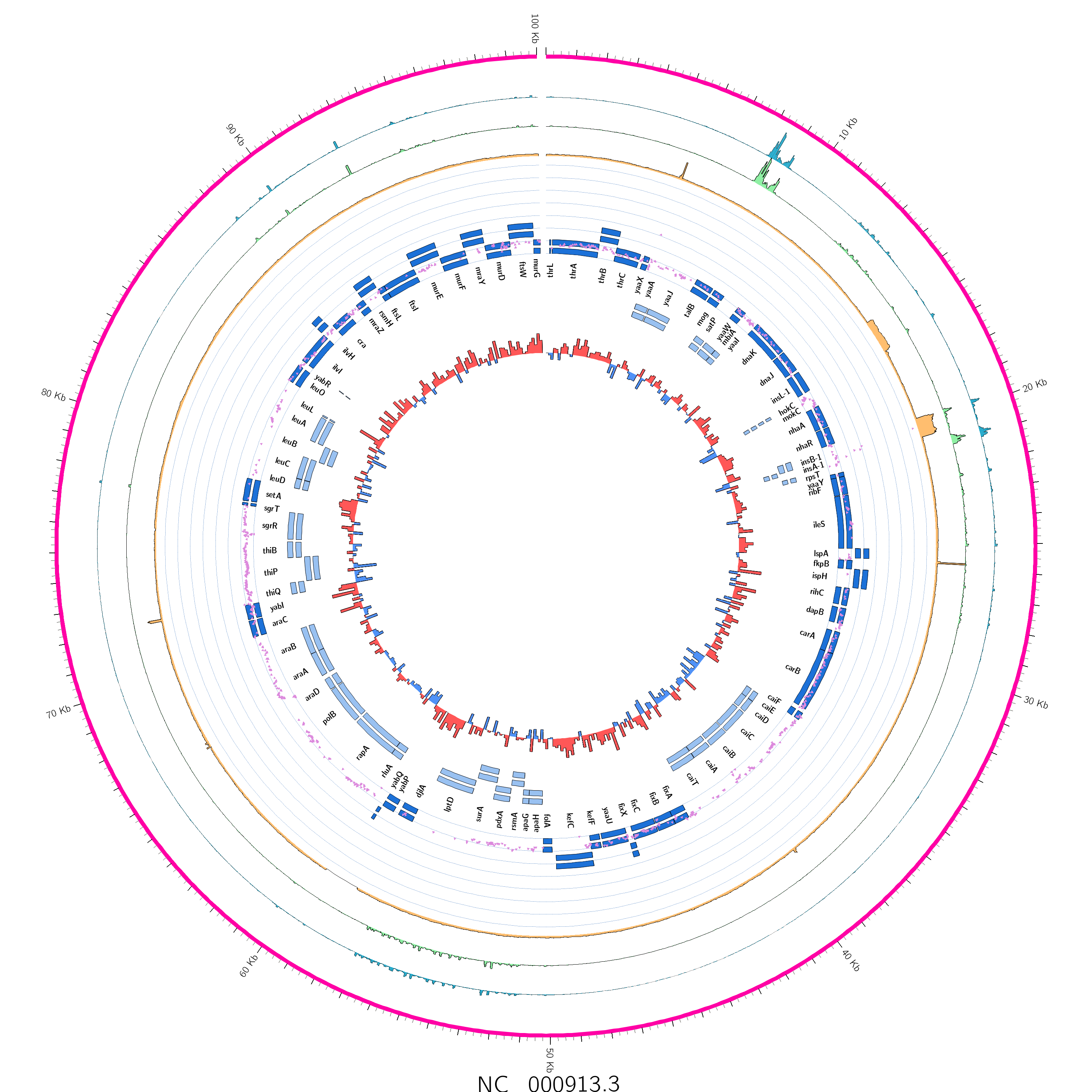
Making the Plot
With our:
gene calls
variant calls
and sequencing depth
We’re ready to run Circos! As this is a ‘near-final’ circos plot it’s requires complicated configuration. Normally you would reach configuration like this with a lot of iterations. It took the tutorial author around 20 executions of the Circos tool to produce this plot.
Hands On: Circos
Circos ( Galaxy version 0.69.8+galaxy9) with the following parameters:
In “Karyotype”:
“Reference Genome Source”: ` FASTA File from History (can be slow, generate a length file to improve execution time.)`
param-file“Source FASTA Sequence”: genome.fa (Uploaded dataset)
In “Ideogram”:
“Chromosome units”: Kilobases
“Spacing Between Ideograms (in chromosome units)”: 0.3
“Thickness”: 10.0
In “Labels”:
“Label Font Size”: 48
In “2D Data Tracks”:
In “2D Data Plot”:
param-repeat“Insert 2D Data Plot”
“Outside Radius”: 0.98
“Inside Radius”: 0.92
“Plot Type”: Histogram
param-file“Histogram Data Source”: output of Circos: bigWig to Scatter on RNA Seq Coverage 2 tool
In “Plot Format Specific Options”:
“Fill Color”: #f08fa4
param-repeat“Insert 2D Data Plot”
“Outside Radius”: 0.92
“Inside Radius”: 0.86
“Plot Type”: Histogram
param-file“Histogram Data Source”: output of Circos: bigWig to Scatter on RNA Seq Coverage 1 tool
In “Plot Format Specific Options”:
“Fill Color”: #8ff0a4
param-repeat“Insert 2D Data Plot”
“Outside Radius”: 0.86
“Inside Radius”: 0.8
“Plot Type”: Histogram
param-file“Histogram Data Source”: output of Circos: bigWig to Scatter on DNA sequencing coverage tool
In “Plot Format Specific Options”:
“Fill Color”: #ffbe6f
param-repeat“Insert 2D Data Plot”
“Outside Radius”: 0.79
“Inside Radius”: 0.6
“Z-index”: 10 (This is used to plot over the genes which are added later.)
“Plot Type”: Scatter
param-file“Scatter Data Source”: output of cut on variants.vcf tool
In “Plot Format Specific Options”:
“Glyph”: Triangle
“Glyph Size”: 6
“Fill Color”: #dc8add
“Stroke Thickness”: 0
In “Axes”:
In “Axis”:
param-repeat“Insert Axis”
“Radial Position”: Absolute position (values match data values)
“Spacing”: 5000.0
“y1”: 40000.0
“Color”: #1a5fb4
“Color Transparency”: 0.4
param-repeat“Insert 2D Data Plot”
“Outside Radius”: 0.6
“Inside Radius”: 0.55
“Plot Type”: Text Labels
param-file“Text Data Source”: output of Circos: Interval to Text on genes (NCBI).gff tool
In “Plot Format Specific Options”:
“Label Size”: 18
“Show Link”: No
“Snuggle Labels”: Yes
param-repeat“Insert 2D Data Plot”
“Outside Radius”: 0.7
“Inside Radius”: 0.6
“Plot Type”: Tiles
param-file“Tile Data Source”: output of Circos: Interval to Tiles on genes (NCBI).gff tool
In “Plot Format Specific Options”:
“Fill Color”: #1c71d8
“Overflow Behavior”: Hide: overflow tiles are not drawn
In “Rules”:
In “Rule”:
param-repeat“Insert Rule”
In “Conditions to Apply”:
param-repeat“Insert Conditions to Apply”
“Condition”: Based on qualifier value (when available)
“Qualifier name”: strand
“Condition”: Less than (numeric)
“Qualifier value to compare against”: 0
In “Actions to Apply”:
param-repeat“Insert Actions to Apply”
“Action”: Change Visibility
param-repeat“Insert 2D Data Plot”
“Outside Radius”: 0.53
“Inside Radius”: 0.45
“Plot Type”: Tiles
param-file“Tile Data Source”: output of Circos: Interval to Tiles on genes (NCBI).gff tool
In “Plot Format Specific Options”:
“Overflow Behavior”: Hide: overflow tiles are not drawn
“Orient Inwards”: Yes
In “Rules”:
In “Rule”:
param-repeat“Insert Rule”
In “Conditions to Apply”:
param-repeat“Insert Conditions to Apply”
“Condition”: Based on qualifier value (when available)
“Qualifier name”: strand
“Condition”: Greater than (numeric)
“Qualifier value to compare against”: 0
In “Actions to Apply”:
param-repeat“Insert Actions to Apply”
“Action”: Change Visibility
param-repeat“Insert Rule”
In “Conditions to Apply”:
param-repeat“Insert Conditions to Apply”
“Condition”: Apply to Every Point
In “Actions to Apply”:
param-repeat“Insert Actions to Apply”
“Action”: Change Fill Color for all points
“Fill Color”: #99c1f1
param-repeat“Insert 2D Data Plot”
“Outside Radius”: 0.45
“Inside Radius”: 0.35
“Plot Type”: Histogram
param-file“Histogram Data Source”: output of Circos: bigWig to Scatter on the GC Skew Plot tool
In “Plot Format Specific Options”:
“Fill Color”: #ff5757
In “Rules”:
In “Rule”:
param-repeat“Insert Rule”
In “Conditions to Apply”:
param-repeat“Insert Conditions to Apply”
“Condition”: Based on value (ONLY for scatter/histogram/heatmap/line)
“Points below this value”: 0.0
In “Actions to Apply”:
param-repeat“Insert Actions to Apply”
“Action”: Change Fill Color for all points
“Fill Color”: #5092f7
In “Ticks”:
“Skip first label”: Yes
In “Tick Group”:
param-repeat“Insert Tick Group”
“Tick Spacing”: 10.0
“Tick Size”: 20.0
“Show Tick Labels”: Yes
param-repeat“Insert Tick Group”
“Tick Size”: 15.0
“Show Tick Labels”: No
param-repeat“Insert Tick Group”
“Tick Spacing”: 0.25
“Color”: #9a9996
“Show Tick Labels”: No
Comment: Circos is complicated
Please check your parameters carefully, and expect that mistakes can be made. Just re-run the tool and modify your parameters!
And while this example is probably very overwhelming, when you create a
Circos plot from scratch, it will be less overwhelming; it’ll be your
data which you know better, and you’ll add one track at a time.
Congratulations on plotting a microbial genome subset in Circos!
Conclusion
Plotting with Circos is essentially infinitely customisable but here we offer suggestions for a default plotting workflow.
reduced for faster plotting and faster data download ↩
You've Finished the Tutorial
Please also consider filling out the Feedback Form as well!
Key points
Circos is incredibly customisable
Not all customisations have to be done with rules, but they can be a useful method
Frequently Asked Questions
Have questions about this tutorial? Have a look at the available FAQ pages and support channels
Did you use this material as an instructor? Feel free to give us feedback on how it went.
Did you use this material as a learner or student? Click the form below to leave feedback.
Hiltemann, Saskia, Rasche, Helena et al., 2023 Galaxy Training: A Powerful Framework for Teaching! PLOS Computational Biology 10.1371/journal.pcbi.1010752
Batut et al., 2018 Community-Driven Data Analysis Training for Biology Cell Systems 10.1016/j.cels.2018.05.012
@misc{visualisation-circos-microbial,
author = "Helena Rasche",
	title = "Ploting a Microbial Genome with Circos (Galaxy Training Materials)",
	year = "",
	month = "",
	day = "",
	url = "\url{https://training.galaxyproject.org/training-material/topics/visualisation/tutorials/circos-microbial/tutorial.html}",
	note = "[Online; accessed TODAY]"
}
@article{Hiltemann_2023,
	doi = {10.1371/journal.pcbi.1010752},
	url = {https://doi.org/10.1371%2Fjournal.pcbi.1010752},
	year = 2023,
	month = {jan},
	publisher = {Public Library of Science ({PLoS})},
	volume = {19},
	number = {1},
	pages = {e1010752},
	author = {Saskia Hiltemann and Helena Rasche and Simon Gladman and Hans-Rudolf Hotz and Delphine Larivi{\`{e}}re and Daniel Blankenberg and Pratik D. Jagtap and Thomas Wollmann and Anthony Bretaudeau and Nadia Gou{\'{e}} and Timothy J. Griffin and Coline Royaux and Yvan Le Bras and Subina Mehta and Anna Syme and Frederik Coppens and Bert Droesbeke and Nicola Soranzo and Wendi Bacon and Fotis Psomopoulos and Crist{\'{o}}bal Gallardo-Alba and John Davis and Melanie Christine Föll and Matthias Fahrner and Maria A. Doyle and Beatriz Serrano-Solano and Anne Claire Fouilloux and Peter van Heusden and Wolfgang Maier and Dave Clements and Florian Heyl and Björn Grüning and B{\'{e}}r{\'{e}}nice Batut and},
	editor = {Francis Ouellette},
	title = {Galaxy Training: A powerful framework for teaching!},
	journal = {PLoS Comput Biol}
}
Funding
These individuals or organisations provided funding support for the development of this resource
5 stars:
Liked: It looks really useful, clearly explained. I still didn`t get it to work with my own data, but I am just learning.
Disliked: I believe the link to the workflow is incorrect, it links to something else
Questions:


 Open image in new tab