Identification of AMR genes in an assembled bacterial genome
| Author(s) |
|
| Editor(s) |
|
| Reviewers |
|
OverviewQuestions:
Objectives:
Which resistance genes are on a bacterial genome?
Where are the genes located on the genome?
Requirements:
Run a series of tool to assess the presence of antimicrobial resistance genes (ARG)
Get information about ARGs
Visualize the ARGs and plasmid genes in their genomic context
Time estimation: 2 hoursLevel: Introductory IntroductorySupporting Materials:Published: Jan 23, 2024Last modification: Dec 18, 2025License: Tutorial Content is licensed under Creative Commons Attribution 4.0 International License. The GTN Framework is licensed under MITpurl PURL: https://gxy.io/GTN:T00401rating Rating: 4.0 (0 recent ratings, 5 all time)version Revision: 10
Antimicrobial resistance (AMR) is a global phenomenon with no geographical or species boundaries, which poses an important threat to human, animal and environmental health. It is a complex and growing problem that compromises our ability to treat bacterial infections.
AMR gene content can be assessed from whole genome sequencing to detect known resistance mechanisms and potentially identify novel mechanisms.
To illustrate the process to identify AMR gene in a bacterial genome, we take an assembly of a bacterial genome (KUN1163 sample) generated by following a bacterial genome assembly tutorial from data produced in “Complete Genome Sequences of Eight Methicillin-Resistant Staphylococcus aureus Strains Isolated from Patients in Japan” (Hikichi et al. 2019).
Methicillin-resistant Staphylococcus aureus (MRSA) is a major pathogen causing nosocomial infections, and the clinical manifestations of MRSA range from asymptomatic colonization of the nasal mucosa to soft tissue infection to fulminant invasive disease. Here, we report the complete genome sequences of eight MRSA strains isolated from patients in Japan.
AgendaIn this tutorial, we will cover:
Galaxy and data preparation
Any analysis should get its own Galaxy history. So let’s start by creating a new one and get the data (contig file from the assembly) into it.
Hands On: Prepare Galaxy and data
Create a new history for this analysis
To create a new history simply click the new-history icon at the top of the history panel:
Rename the history
- Click on galaxy-pencil (Edit) next to the history name (which by default is “Unnamed history”)
- Type the new name
- Click on Save
- To cancel renaming, click the galaxy-undo “Cancel” button
If you do not have the galaxy-pencil (Edit) next to the history name (which can be the case if you are using an older version of Galaxy) do the following:
- Click on Unnamed history (or the current name of the history) (Click to rename history) at the top of your history panel
- Type the new name
- Press Enter
Import the contig file from Zenodo or from Galaxy shared data libraries:
https://zenodo.org/record/10572227/files/DRR187559_contigs.fasta
- Copy the link location
Click galaxy-upload Upload at the top of the activity panel
- Select galaxy-wf-edit Paste/Fetch Data
Paste the link(s) into the text field
Press Start
- Close the window
As an alternative to uploading the data from a URL or your computer, the files may also have been made available from a shared data library:
- Go into Libraries (left panel)
- Navigate to the correct folder as indicated by your instructor.
- On most Galaxies tutorial data will be provided in a folder named GTN - Material –> Topic Name -> Tutorial Name.
- Select the desired files
- Click on Add to History galaxy-dropdown near the top and select as Datasets from the dropdown menu
In the pop-up window, choose
- “Select history”: the history you want to import the data to (or create a new one)
- Click on Import


Identification of AMR genes
To identify AMR genes in contigs, tools like ABRicate or staramr (Bharat et al. 2022) can be used. In this tutorial, we use staramr. Staramr scans bacterial genome contigs against the ResFinder (Zankari et al. 2012), PointFinder (Zankari et al. 2017), and PlasmidFinder (Carattoli et al. 2014) databases (used by the ResFinder webservice) and compiles a summary report of detected antimicrobial resistance genes.
CommentIf you are interested in learning more about using ABRicate for AMR gene detection, you can check the sub-section on AMR in “Gene based pathogenic identification” of “Pathogen detection from (direct Nanopore) sequencing data using Galaxy - Foodborne Edition” tutorial
Hands On: Run staramr
- staramr ( Galaxy version 0.10.0+galaxy1) with the following parameters:
- param-file “genomes”: Contig file
staramr generates 8 outputs:
-
summary.tsv: A summary of all detected AMR genes/mutations/plasmids/sequence type in each genome, one genome per line and the following columns:- Isolate ID: The id of the isolate/genome file(s) passed to
staramr. - Quality Module: The isolate/genome file(s) pass/fail result(s) for the quality metrics
- Genotype: The AMR genotype of the isolate.
- Predicted Phenotype: The predicted AMR phenotype (drug resistances) for the isolate.
-
CGE Predicted Phenotype: The CGE-predicted AMR phenotype (drug resistances) for the isolate (CGE = Center for Genomic Epidemiology)
- Plasmid: Plasmid types that were found for the isolate.
-
Scheme: The MLST scheme used
MLST stands for MultiLocus Sequence Typing. It is a technique for the typing of multiple loci, using DNA sequences of internal fragments of multiple housekeeping genes to characterize isolates of microbial species.
Here, starmr uses mlst to scan the contig files against traditional PubMLST typing schemes. The correspondance between the scheme and the bacteria genus and species is accessible in the map
- Sequence Type: The sequence type that’s assigned when combining all allele types
- Genome Length: The isolate/genome file(s) genome length(s)
- N50 value: The isolate/genome file(s) N50 value(s)
- Number of Contigs Greater Than Or Equal To 300 bp: The number of contigs greater or equal to 300 base pair in the isolate/genome file(s)
- Quality Module Feedback: The isolate/genome file(s) detailed feedback for the quality metrics
Hands On: Inspect the staramr output- View galaxy-eye the
summary.tsvfile
Question: Inspect the staramr output- How many genomes are there?
- Has the genome failed or passed the quality? Why?
- What are the predicted AMR drug resistances? Are they similar to the one found for KUN1163 in Table 1 in Hikichi et al. 2019?
- What is the MLST scheme? Does that correspond to the expected species and genus?
- There is one genome (1 line)
- The genome has failed the quality (column 2), because the genome length is not within the acceptable length range (last column).
-
We can summarize starmr output and Table 1 in Hikichi et al. 2019:
Antibiotic name Abbreviation staramr Hikichi et al. 2019 Amikacin Yes Azithromycin Yes Cefazolin CEZ Yes clindamycin CLDM Yes Erythromycin EM Yes Yes Gentamicin GM Yes Yes Imipenem IPM Yes Levofloxacin LVFX Yes Oxacillin MPIPC Yes Penicillin Yes Spectinomycin Yes Tetracycline Yes Tobramycin Yes - The scheme is saureus, so Staphylococcus aureus (given the scheme genus map), which is coherent with MRSA
- Isolate ID: The id of the isolate/genome file(s) passed to
-
detailed_summary.tsv: A detailed summary of all detected AMR genes/mutations/plasmids/sequence type in each genome, one gene per line and the following columns:- Isolate ID: The id of the isolate/genome file(s) passed to
staramr. - Data: The particular gene detected from ResFinder, PlasmidFinder, PointFinder, or the sequence type.
- Data Type: The type of gene (Resistance or Plasmid), or MLST.
- Predicted Phenotype: The predicted AMR phenotype (drug resistances) found in ResFinder/PointFinder. Plasmids will be left blank by default.
- CGE Predicted Phenotype: The CGE-predicted AMR phenotype (drug resistances) found in ResFinder/PointFinder. Plasmids will be left blank by default.
- %Identity: The % identity of the top BLAST HSP to the gene.
- %Overlap: THe % overlap of the top BLAST HSP to the gene (calculated as hsp length/total length * 100).
- HSP Length/Total Length The top BLAST HSP length over the gene total length (nucleotides).
- Contig: The contig id containing this gene.
- Start: The start of the gene (will be greater than End if on minus strand).
- End: The end of the gene.
- Accession: The accession of the gene from either ResFinder or PlasmidFinder database.
Hands On: Inspect the staramr output- View galaxy-eye the
detailed_summary.tsvfile
Question: Inspect the staramr output- What are the different sequence types that have been identified?
- Where are located the plasmid genes?
- Where are located the resistances genes?
- By looking for the accession number (M13771) on NCBI (https://www.ncbi.nlm.nih.gov/nuccore/), where does the first resistance come from?
- There are:
- 1 MSLT
- 5 plasmid rep genes
- 7 resistance genes
- The plasmid genes are on contig00019 (3 genes - coherent with Lozano et al. 2012), contig00024, and contig00002.
- The resistance genes are:
- 4/7 on contigs with plasmid genes (contig00002, contig00019, contig00024)
- 3/7 on contigs without plasmid genes (contig00022, contig00021)
- M13771 is a 6’-aminoglycoside acetyltransferase phosphotransferase (AAC(6’)-APH(2’)) bifunctional resistance protein from Streptococcus faecalis. It might come from horizontal transfer from Streptococcus faecalis on a plasmid of Staphylococcus aureus.
- Isolate ID: The id of the isolate/genome file(s) passed to
-
resfinder.tsv: A tabular file of each AMR gene and additional BLAST information from the ResFinder database, one gene per line and the following columns:- Isolate ID: The id of the isolate/genome file(s) passed to
staramr. - Gene: The particular AMR gene detected.
- Predicted Phenotype: The predicted AMR phenotype (drug resistances) for this gene.
- CGE Predicted Phenotype: The CGE-predicted AMR phenotype (drug resistances) for this gene.
- %Identity: The % identity of the top BLAST HSP to the AMR gene.
- %Overlap: THe % overlap of the top BLAST HSP to the AMR gene (calculated as hsp length/total length * 100).
- HSP Length/Total Length The top BLAST HSP length over the AMR gene total length (nucleotides).
- Contig: The contig id containing this AMR gene.
- Start: The start of the AMR gene (will be greater than End if on minus strand).
- End: The end of the AMR gene.
- Accession: The accession of the AMR gene in the ResFinder database.
- Sequence: The AMR Gene sequence
- CGE Notes: Any CGE notes associated with the prediction.
- Isolate ID: The id of the isolate/genome file(s) passed to
-
plasmidfinder.tsv: A tabular file of each AMR plasmid type and additional BLAST information from the PlasmidFinder database, one plasmid type per line with the following columns:- Isolate ID: The id of the isolate/genome file(s) passed to
staramr. - Plasmid: The particular plasmid type detected.
- %Identity: The % identity of the top BLAST HSP to the plasmid type.
- %Overlap: The % overlap of the top BLAST HSP to the plasmid type (calculated as hsp length/total length * 100).
- HSP Length/Total Length The top BLAST HSP length over the plasmid type total length (nucleotides).
- Contig: The contig id containing this plasmid type.
- Start: The start of the plasmid type (will be greater than End if on minus strand).
- End: The end of the plasmid type.
- Accession: The accession of the plasmid type in the PlasmidFinder database.
- Isolate ID: The id of the isolate/genome file(s) passed to
-
mlst.tsv: A tabular file of each multi-locus sequence type (MLST) and it’s corresponding locus/alleles, one genome per line with the following columns:- Isolate ID: The id of the isolate/genome file(s) passed to
staramr. - Scheme: The scheme that
MLSThas identified. - Sequence Type: The sequence type that’s assigned when combining all allele types
- Locus #: A particular locus in the specified MLST scheme.
- Isolate ID: The id of the isolate/genome file(s) passed to
settings.txt: The command-line, database versions, and other settings used to runstaramr.results.xlsx: An Excel spreadsheet containing the previous files as separate worksheets.hits: A collection with fasta files of the BLAST HSP nucleotides for the entries listed in the resfinder.tsv and pointfinder.tsv files. There are up to two files per input genome, one for ResFinder and one for PointFinder.
Getting more information about ARG via the CARD database
To get more information about the antibiotic resistant genes (ARG), we can check the CARD database (Comprehensive Antibiotic Resistance Database) (Jia et al. 2016)
CARD can be very helpful to check all the resistance genes and check if it is logical to find the resistance gene in a specific bacteria.
Question
- To what family does mecA belong?
- Do you expect to find this gene in this MRSA strain and why?
- Is the accession number of the entry related to the accession reported by staramr?
- Methicillin resistant PBP2
- The strain we use is a Methicillin(multi) resistant Staphylococcus aureus. As
mecAhas a perfect resistome mach with S. aureus, and the AMR Gene Family is methicillin resistant PBP2, we expect to see mecA in MRSA.- No, these are completely unrelated. Unfortunately this is a very common issue in bioinformatics. Everyone builds their own numbering system for entries in their database (usually calling them ‘accessions’), and then someone else needs to build a service to link these databases.
Visualization of the ARGs and plasmid genes in their genomic context
We would like to look at the ARGs and plasmid genes in their genomic context. To do that, we will usie JBrowse (Diesh et al. 2023) with several information:
- Assembly as the reference
- ARGs location
- Contigs annotation (genes, etc)
- Coverage of the contigs from the raw reads
Extraction of the ARG and plasmid genes location
The first step is to extract the location of the ARGs and plasmid genes on the contigs. This information is available on the detailed_summary.tsv output of starmar. The genes and their location are on the lines with a decimal value on column 6 or 7. So to only get this information, we need to select lines with a decimal value (###.##) followed by a tab character, the column separator in Galaxy. As a result, any lines without an identity or overlap value will be filtered out.
Hands On: Extract ARGs and plasmid genes
- Select lines that match an expression with the following parameters:
- param-file “Select lines from”:
detailed_summary.tsvstaramr output- “that”: Matching
- “the pattern”:
[0-9]+\.[0-9]+\t
QuestionHow many genes have been kept?
12
This table can not be used directly in JBrowse. It first needs to be transformed in a standard format: GFF3, a file format used for describing genes and other features of DNA, RNA and protein sequences.
Comment: GFF3 file formatA GFF is a tab delimited file with 9 fields per line:
- seqid: The name of the sequence where the feature is located.
- source: The algorithm or procedure that generated the feature. This is typically the name of a software or database.
- type: The feature type name, like “gene” or “exon”. In a well structured GFF file, all the children features always follow their parents in a single block (so all exons of a transcript are put after their parent “transcript” feature line and before any other parent transcript line). In GFF3, all features and their relationships should be compatible with the standards released by the Sequence Ontology Project.
- start: Genomic start of the feature, with a 1-base offset. This is in contrast with other 0-offset half-open sequence formats, like BED.
- end: Genomic end of the feature, with a 1-base offset. This is the same end coordinate as it is in 0-offset half-open sequence formats, like BED.
- score: Numeric value that generally indicates the confidence of the source in the annotated feature. A value of “.” (a dot) is used to define a null value.
- strand: Single character that indicates the strand of the feature. This can be “+” (positive, or 5’->3’), “-“, (negative, or 3’->5’), “.” (undetermined), or “?” for features with relevant but unknown strands.
- phase: phase of CDS features; it can be either one of 0, 1, 2 (for CDS features) or “.” (for everything else). See the section below for a detailed explanation.
- attributes: A list of tag-value pairs separated by a semicolon with additional information about the feature.
Hands On: Create a GFF file
- Table to GFF3 ( Galaxy version 1.2)
- param-file “Table”: output of the above Select lines tool step
- “Record ID column or value”:
9- “Start column or value”:
10- “End column or value”:
11- “Type column or value”:
3- “Score column or value”:
6- “Source column or value”:
3- param-repeat “Insert Qualifiers”
- “Name”:
name- “Qualifier value column or raw text”:
2- param-repeat “Insert Qualifiers”
- “Name”:
phenotype- “Qualifier value column or raw text”:
4- param-repeat “Insert Qualifiers”
- “Name”:
accession- “Qualifier value column or raw text”:
12
QuestionHow many genes have been found per contigs?
- Contig 19: 3 plasmid genes, 1 ARG
- Contig 24: 1 plasmid gene, 2 ARGs
- Contig 2: 1 plasmid gene, 1 ARG
- Contig 22: 2 ARGs
- Contig 21: 1 ARG
Annotation of the contigs
In addition to the ARGs and plasmid genes, it would be good to have extra information about other genes on the contigs. Several tools exists to do that: Prokka (Seemann 2014), Bakta (Schwengers et al. 2021), etc. Here, we use Bakta as recommended by Torsten Seeman as the successor of Prokka.
Hands-on: Choose Your Own TutorialThis is a 'Choose Your Own Tutorial' (CYOT) section (also known as 'Choose Your Own Analysis' (CYOA)), where you can select between multiple paths. Click one of the buttons below to select how you want to follow the tutorial
Have you already run Bakta on this dataset before?
Bakta is a tool for the rapid & standardized annotation of bacterial genomes and plasmids from both isolates and MAGs.
Hands On: Annotate the contigs
- Bakta ( Galaxy version 1.8.2+galaxy0) with the following parameters:
- In “Input/Output options”:
- “The bakta database”: latest one
- “The amrfinderplus database”: latest one
- param-file “Select genome in fasta format”: Contig file
- In “Optional annotation”:
- “Keep original contig header (–keep-contig-headers)”:
Yes
QuestionHow many features have been identified?
51k+ (number of lines in the GFF)
If you already ran Bakta on your contigs, you can just upload here the GFF generated by Bakta.
Hands On: Import annotation GFF
- Import the GFF file generated by Bakta

Mapping the raw reads on the contigs
To get information about the coverage of the contigs and genes, we map the reads used to build the contigs to the contigs using Bowtie2 (Langmead et al. 2009).
Hands On: Annotating the Genome
Import the reads (after quality control) from another history, from Zenodo or from Galaxy shared data libraries:
https://zenodo.org/record/10572227/files/DRR187559_after_fastp_1.fastq.gz
https://zenodo.org/record/10572227/files/DRR187559_after_fastp_2.fastq.gz
Create a paired collection named
Paired Reads
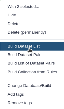
- Click on galaxy-selector Select Items at the top of the history panel
- Check all the datasets in your history you would like to include
Click n of N selected and choose Advanced Build List
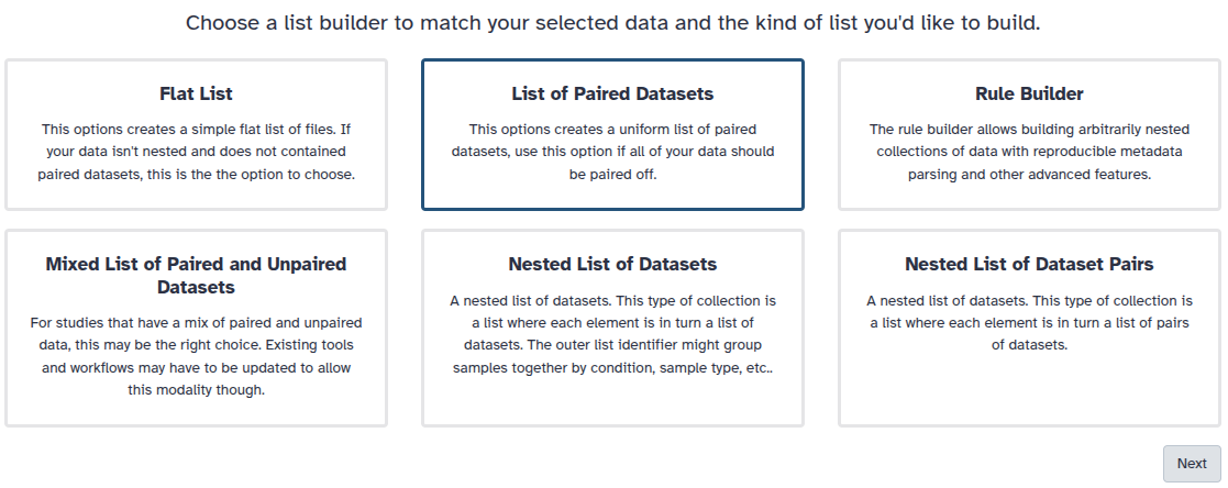
You are in the collection building wizard. Choose List of Paired Datasets and click ‘Next’ button at the right bottom corner.
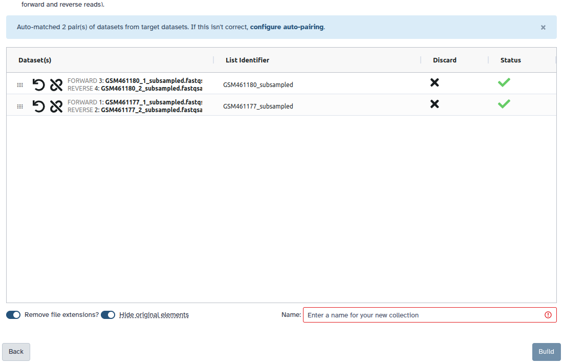
Check and configure auto-pairing. Commonly matepairs have suffix
_1and_2or_R1and_R2. Click on ‘Next’ at the bottom.
- Edit the List Identifier as required.
- Enter a name for your collection
- Click Build to build your collection
- Click on the checkmark icon at the top of your history again
Bowtie2 ( Galaxy version 2.5.4+galaxy0) with the following parameters:
- “Is this single or paired library”:
Paired-end
- param-collection “FASTQ Paired Dataset”:
Paired Reads- “Will you select a reference genome from your history or use a built-in index?”:
Use a genome from the history and build index
- param-file “Select reference genome”: Contig file
- “Save the bowtie2 mapping statistics to the history”:
Yes

QuestionWhat is the alignment rate? What does that mean for the assembly?
The alignment rate is 99.77%. Most of the reads have been mapped on the contigs. They have been then used to build the contigs.
Visualisation of the ARGs
We can now visualize the contigs, the mapping coverage, and the genes, using JBrowse and different information track.
Hands On: Visualize the Genome
- JBrowse ( Galaxy version 1.16.11+galaxy1) with the following parameters:
- “Reference genome to display”:
Use a genome from history
- param-file “Select the reference genome”: Contig file
- “Genetic Code”:
11. The Bacterial, Archaeal and Plant Plastid Code- In “Track Group”:
- param-repeat “Insert Track Group”
- “Track Category”:
Bakta- In “Annotation Track”:
- param-repeat “Insert Annotation Track”
- “Track Type”:
GFF/GFF3/BED Features
- param-file “GFF/GFF3/BED Track Data”:
Annotation_and_sequences(output of Bakta tool)- “JBrowse Track Type [Advanced]”:
Neat Canvas Features- “Track Visibility”:
On for new users- param-repeat “Insert Track Group”
- “Track Category”:
ARGs and plasmid genes- In “Annotation Track”:
- param-repeat “Insert Annotation Track”
- “Track Type”:
GFF/GFF3/BED Features
- param-file “GFF/GFF3/BED Track Data”: Output of Table to GFF3
- “JBrowse Track Type [Advanced]”:
Neat Canvas Features- “Track Visibility”:
On for new users- param-repeat “Insert Track Group”
- “Track Category”:
Coverage- In “Annotation Track”:
- param-repeat “Insert Annotation Track”
- “Track Type”:
BAM Pileups
- param-file “BAM Track Data”: Bowtie2’s output
- “Autogenerate SNP Track”:
Yes- View the output of JBrowse
In the output of the JBrowse you can view the mapped reads and the found genes against the reference genome. With the search tools you can easily find genes of interest. JBrowse can handle many inputs and can be very useful. Using the Bowtie2 mapping output, low coverage regions can be detected. This SNP detection can also give a clear view of where the data was less reliable or where variations were located.
If it takes too long to build the JBrowse instance, you can view an embedded one here. (Warning: feature name search will not work.)
Question
- What is the name for the gene found by Bakta corresponding to the rep16 gene found by staramr?
- What are the NCBI Protein id and UniRef id for aac(6’)-aph(2’’)?
- By zooming at the beginning of the contig, the name for rep16 is DUF536 domain-containing protein
- aac(6’)-aph(2’’) is on contig00019:20311..21749. The corresponding gene found by Bakta is bifunctional aminoglycoside N-acetyltransferase AAC(6’)-Ie/aminoglycoside O-phosphotransferase APH(2’’)-Ia. When clicking on it, we can find the dbxref attributes:
- NCBI Protein: WP_001028144.1
- UniRef: UniRef50_P0A0C2
Conclusion
In this tutorial, contigs were scaned for AMR and plasmid genes. The genes were then visualized in their genomic context after contig annotation.
You've Finished the Tutorial
Key points
staramr is a powerful tool to predict ARGs and plasmid genes
Visualization of the ARGs and plasmid genes in their genomic context helps to make sense of the data
Frequently Asked Questions
Have questions about this tutorial? Have a look at the available FAQ pages and support channelsReferences
- Langmead, B., C. Trapnell, M. Pop, and S. L. Salzberg, 2009 Ultrafast and memory-efficient alignment of short DNA sequences to the human genome. Genome biology 10: 1–10. 10.1186/gb-2009-10-3-r25
- Lozano, C., Garcı́a-Migura Lourdes, C. Aspiroz, M. Zarazaga, C. Torres et al., 2012 Expansion of a Plasmid Classification System for Gram-Positive Bacteria and Determination of the Diversity of Plasmids in Staphylococcus aureus Strains of Human, Animal, and Food Origins. Applied and Environmental Microbiology 78: 5948–5955. 10.1128/aem.00870-12
- Zankari, E., H. Hasman, S. Cosentino, M. Vestergaard, S. Rasmussen et al., 2012 Identification of acquired antimicrobial resistance genes. Journal of antimicrobial chemotherapy 67: 2640–2644. 10.1093/jac/dks261
- Carattoli, A., E. Zankari, Garcı̀a-Fernandez Aurora, M. V. Larsen, O. Lund et al., 2014 In silico detection and typing of plasmids using PlasmidFinder and plasmid multilocus sequence typing . Antimicrob Agents Chemother 58: 3895–903. 10.1128/AAC.02412-14 0
- Seemann, T., 2014 Prokka: rapid prokaryotic genome annotation. Bioinformatics 30: 2068–2069. 10.1093/bioinformatics/btu153
- Jia, B., A. R. Raphenya, B. Alcock, N. Waglechner, P. Guo et al., 2016 CARD 2017: expansion and model-centric curation of the comprehensive antibiotic resistance database. Nucleic Acids Research 45: D566–D573. 10.1093/nar/gkw1004
- Zankari, E., R. Allesøe, K. G. Joensen, L. M. Cavaco, O. Lund et al., 2017 PointFinder: a novel web tool for WGS-based detection of antimicrobial resistance associated with chromosomal point mutations in bacterial pathogens. Journal of Antimicrobial Chemotherapy 72: 2764–2768. 10.1093/jac/dkx217
- Hikichi, M., M. Nagao, K. Murase, C. Aikawa, T. Nozawa et al., 2019 Complete Genome Sequences of Eight Methicillin-Resistant Staphylococcus aureus Strains Isolated from Patients in Japan (I. L. G. Newton, Ed.). Microbiology Resource Announcements 8: 10.1128/mra.01212-19
- Schwengers, O., L. Jelonek, M. A. Dieckmann, S. Beyvers, J. Blom et al., 2021 Bakta: rapid and standardized annotation of bacterial genomes via alignment-free sequence identification. Microbial genomics 7: 000685. 10.1099/mgen.0.000685
- Bharat, A., A. Petkau, B. P. Avery, J. C. Chen, J. P. Folster et al., 2022 Correlation between phenotypic and in silico detection of antimicrobial resistance in Salmonella enterica in Canada using Staramr. Microorganisms 10: 292. 10.3390/microorganisms10020292
- Diesh, C., G. J. Stevens, P. Xie, T. De Jesus Martinez, E. A. Hershberg et al., 2023 JBrowse 2: a modular genome browser with views of synteny and structural variation. Genome biology 24: 1–21. 10.1186/s13059-023-02914-z
Feedback
Did you use this material as an instructor? Feel free to give us feedback on how it went.
Did you use this material as a learner or student? Click the form below to leave feedback.

Citing this Tutorial
- Bazante Sanders, Bérénice Batut, Identification of AMR genes in an assembled bacterial genome (Galaxy Training Materials). https://training.galaxyproject.org/training-material/topics/genome-annotation/tutorials/amr-gene-detection/tutorial.html Online; accessed TODAY
- Hiltemann, Saskia, Rasche, Helena et al., 2023 Galaxy Training: A Powerful Framework for Teaching! PLOS Computational Biology 10.1371/journal.pcbi.1010752
- Batut et al., 2018 Community-Driven Data Analysis Training for Biology Cell Systems 10.1016/j.cels.2018.05.012
@misc{genome-annotation-amr-gene-detection,
author = "Bazante Sanders and Bérénice Batut",
	title = "Identification of AMR genes in an assembled bacterial genome (Galaxy Training Materials)",
	year = "",
	month = "",
	day = "",
	url = "\url{https://training.galaxyproject.org/training-material/topics/genome-annotation/tutorials/amr-gene-detection/tutorial.html}",
	note = "[Online; accessed TODAY]"
}
@article{Hiltemann_2023,
	doi = {10.1371/journal.pcbi.1010752},
	url = {https://doi.org/10.1371%2Fjournal.pcbi.1010752},
	year = 2023,
	month = {jan},
	publisher = {Public Library of Science ({PLoS})},
	volume = {19},
	number = {1},
	pages = {e1010752},
	author = {Saskia Hiltemann and Helena Rasche and Simon Gladman and Hans-Rudolf Hotz and Delphine Larivi{\`{e}}re and Daniel Blankenberg and Pratik D. Jagtap and Thomas Wollmann and Anthony Bretaudeau and Nadia Gou{\'{e}} and Timothy J. Griffin and Coline Royaux and Yvan Le Bras and Subina Mehta and Anna Syme and Frederik Coppens and Bert Droesbeke and Nicola Soranzo and Wendi Bacon and Fotis Psomopoulos and Crist{\'{o}}bal Gallardo-Alba and John Davis and Melanie Christine Föll and Matthias Fahrner and Maria A. Doyle and Beatriz Serrano-Solano and Anne Claire Fouilloux and Peter van Heusden and Wolfgang Maier and Dave Clements and Florian Heyl and Björn Grüning and B{\'{e}}r{\'{e}}nice Batut and},
	editor = {Francis Ouellette},
	title = {Galaxy Training: A powerful framework for teaching!},
	journal = {PLoS Comput Biol}
}
Funding
These individuals or organisations provided funding support for the development of this resource


Do you want to extend your knowledge?Follow one of our recommended follow-up trainings:
You can use Ephemeris's
shed-tools installcommand to install the tools used in this tutorial.shed-tools install [-g GALAXY] [-a API_KEY] -t <(curl https://training.galaxyproject.org/training-material/api/topics/genome-annotation/tutorials/amr-gene-detection/tutorial.json | jq .admin_install_yaml -r)Alternatively you can copy and paste the following YAML
---
install_tool_dependencies: true
install_repository_dependencies: true
install_resolver_dependencies: true
tools:
- name: bowtie2
  owner: devteam
  revisions: f76cbb84d67f
  tool_panel_section_label: Mapping
  tool_shed_url: https://toolshed.g2.bx.psu.edu/
- name: bakta
  owner: iuc
  revisions: 728dacaf08a9
  tool_panel_section_label: Annotation
  tool_shed_url: https://toolshed.g2.bx.psu.edu/
- name: jbrowse
  owner: iuc
  revisions: a6e57ff585c0
  tool_panel_section_label: Graph/Display Data
  tool_shed_url: https://toolshed.g2.bx.psu.edu/
- name: tbl2gff3
  owner: iuc
  revisions: 4a7f4b0cc0a3
  tool_panel_section_label: Annotation
  tool_shed_url: https://toolshed.g2.bx.psu.edu/
- name: staramr
  owner: nml
  revisions: 3b22de20bd4b
  tool_panel_section_label: Metagenomic Analysis
  tool_shed_url: https://toolshed.g2.bx.psu.edu/