DNA Methylation data analysis
| Author(s) |
|
| Editor(s) |
|
| Reviewers |
|
OverviewQuestions:
Objectives:
What is methylation and why it cannot be recognised by a normal NGS procedure?
Can a different methylation influence the expression of a gene? How?
Which tools you can use to analyse methylation data?
Requirements:
Learn how to analyse methylation data
Get a first intuition what are common pitfalls.
- Introduction to Galaxy Analyses
- slides Slides: Quality Control
- tutorial Hands-on: Quality Control
- slides Slides: Mapping
- tutorial Hands-on: Mapping
Time estimation: 3 hoursSupporting Materials:Published: Feb 16, 2017Last modification: Apr 3, 2025License: Tutorial Content is licensed under Creative Commons Attribution 4.0 International License. The GTN Framework is licensed under MITpurl PURL: https://gxy.io/GTN:T00142rating Rating: 3.8 (0 recent ratings, 13 all time)version Revision: 24
We will use a small subset of the original data. If we would do the computation on the orginal data the computation time for a tutorial is too long. To show you all necessary steps for Methyl-Seq we decided to use a subset of the data set. In a second step we use precomputed data from the study to show you different levels of methylation. We will consider samples from normal breast cells (NB), fibroadenoma (noncancerous breast tumor, BT089), two invasive ductal carcinomas (BT126, BT198) and a breast adenocarcinoma cell line (MCF7).
This tutorial is based off of Lin et al. 2015. The data we use in this tutorial is available at Zenodo.
AgendaIn this tutorial, we will deal with:
Data upload
We will start by loading the example dataset which will be used for the tutorial into Galaxy
Hands On: Get the data into Galaxy
Create a new history
To create a new history simply click the new-history icon at the top of the history panel:
Import the two example datasets from Zenodo or the shared data library:
https://zenodo.org/record/557099/files/subset_1.fastq
https://zenodo.org/record/557099/files/subset_2.fastq
- Copy the link location
Click galaxy-upload Upload at the top of the activity panel
- Select galaxy-wf-edit Paste/Fetch Data
Paste the link(s) into the text field
Press Start
- Close the window
As an alternative to uploading the data from a URL or your computer, the files may also have been made available from a shared data library:
- Go into Libraries (left panel)
- Navigate to the correct folder as indicated by your instructor.
- On most Galaxies tutorial data will be provided in a folder named GTN - Material –> Topic Name -> Tutorial Name.
- Select the desired files
- Click on Add to History galaxy-dropdown near the top and select as Datasets from the dropdown menu
In the pop-up window, choose
- “Select history”: the history you want to import the data to (or create a new one)
- Click on Import


Quality Control
The first step in any analysis should always be quality control. We will use the Falco tool to asses the quality of our reads and determine if we need to perform any data cleaning before proceeding with our analysis. Falco is an efficiency optimized rewrite of FastQC
Hands On: Quality Control
- Falco ( Galaxy version 1.2.4+galaxy0) with the following parameters:
- param-files “Raw read data from your current history”:
subset_1.fastq.gzandsubset_2.fastq.gz
- Click on param-files Multiple datasets
- Select several files by keeping the Ctrl (or COMMAND) key pressed and clicking on the files of interest
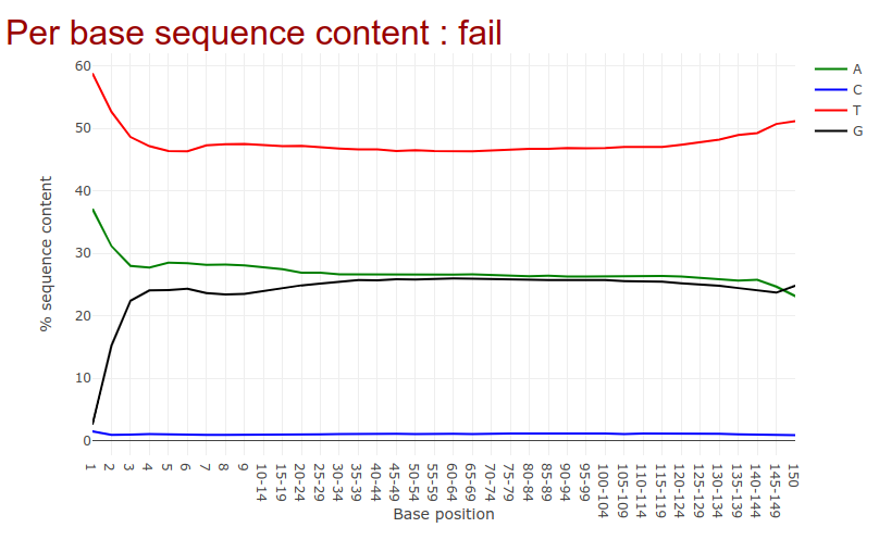
Go to the web page result page and have a closer look at ‘Per base sequence content’
Question
- Note the GC distribution and percentage of “T” and “C”. Why is this so weird?
- Is everything as expected?
- The attentive audience of the theory part knows: Every C-meth stays a C and every normal C becomes a T during the bisulfite conversion.
- Yes it is. Always be careful and have the specific characteristics of your data in mind during the interpretation of Falco results.
Alignment
Hands On: Mapping with bwamethWe will now map the imported dataset against a reference genome.
- bwameth ( Galaxy version 0.2.7+galaxy0) with the following parameters:
- “Select a genome reference from your history or a built-in index?”:
Use a built-in index
- “Select a reference genome”:
Human (hg38full)- “Is this library mate-paired”:
Paired-end
- “First read in pair”:
subset_1.fastq- “Second read in pair”:
subset_2.fastqComment: Long compute timesPlease notice that mapping can take some time. If you want to skip this, we provide for you a precomputed alignment. Import
https://zenodo.org/records/557099/files/aligned_subset.bamto your history.QuestionWhy we need other alignment tools for bisulfite sequencing data?
You may have noticed that all the C’s are C-meth’s and a T can be a T or a C. A mapper for methylation data needs to find out what is what.
Methylation bias and metric extraction
Hands On: Methylation biasIn this step we will have a look at the distribution of the methylation and will look at a possible bias.
- MethylDackel ( Galaxy version 0.5.2+galaxy0) with the following parameters:
- “Load reference genome from”:
Local cache
- “Using reference genome”:
Human (hg38)- “Sorted BAM file”: output of bwameth tool
- “What do you want to do?”:
Determine the position-dependent methylation bias in the dataset, producing diagnostic SVG images (mbias)- In “Advanced options”
- “Keep singletons”: param-toggle
Yes- “Keep discordant alignmetns”: param-toggle
Yes
Question
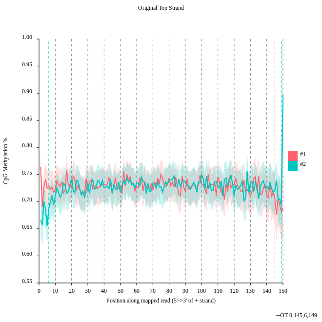
- Consider the
original top strandoutput. Is there a methylation bias?- If we would trim, what would be the start and the end positions?
- The distribution of the methylation is more or less equal. Only at the start and the end we could trim a bit but a +- 5% variation is acceptable.
- To trim the reads we would include for the first strand only the positions 0 to 145, for the second 6 to 149.
Hands On: Methylation extraction with MethylDackelWe will extract the methylation on the resulting BAM file of the alignment step. We need this to create a methylation level plot in the next step.
- MethylDackel ( Galaxy version 0.5.2+galaxy0) with the following parameters:
- “Load reference genome from”:
Local cache
- “Using reference genome”:
Human (hg38)- “Sorted BAM file”: output of bwameth tool
- “What do you want to do?”:
Extract methylation metrics from an alignment file in BAM/CRAM format (extract)- “Merge per-Cytosine metrics”: param-toggle
Yes- “Output options”:
CpG methylation fractions (--fraction)
Visualization
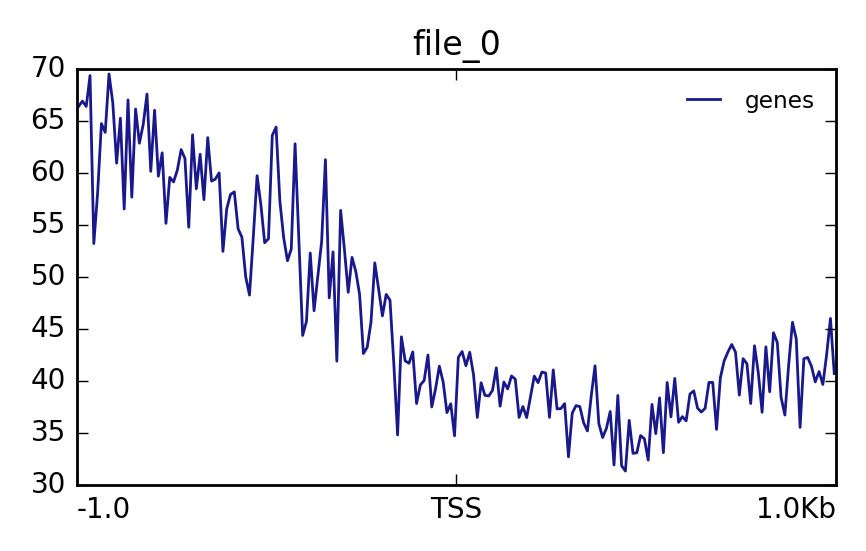
Hands OnIn this step we want to visualize the methylation level around all TSS of our data. When located at gene promoters, DNA methylation is usually a repressive mark.
- Wig/BedGraph-to-bigWig with the following parameters:
“Convert”:
fraction CpG(result of MethylDackel tool)It can happen that you can not select the correct input file. In this case you have to add meta information about the used genome to the file.
- Click on the pencil of the correct history item.
- Change
Database/Build:to the genome you used.- In our case the correct genome is
Human Dec. 2013 (GRCh38/hg38) (hg38).Import the BED file with CpG islands from Zenodo into the history
https://zenodo.org/records/557099/files/CpGIslands.bed- computeMatrix ( Galaxy version 3.5.4+galaxy0) with the following parameters:
- “Regions to plot”:
CpGIslands.bed- “Sample order matters”:
No- “Score file”: Output of Wig/BedGraph-to-bigWig tool
- “computeMatrix has two main output options”:
reference-point- plotProfile ( Galaxy version 3.5.4+galaxy0) with the following parameters:
- “Matrix file from the computeMatrix tool”:
Matrix(output of computeMatrix tool)The output should look like this:
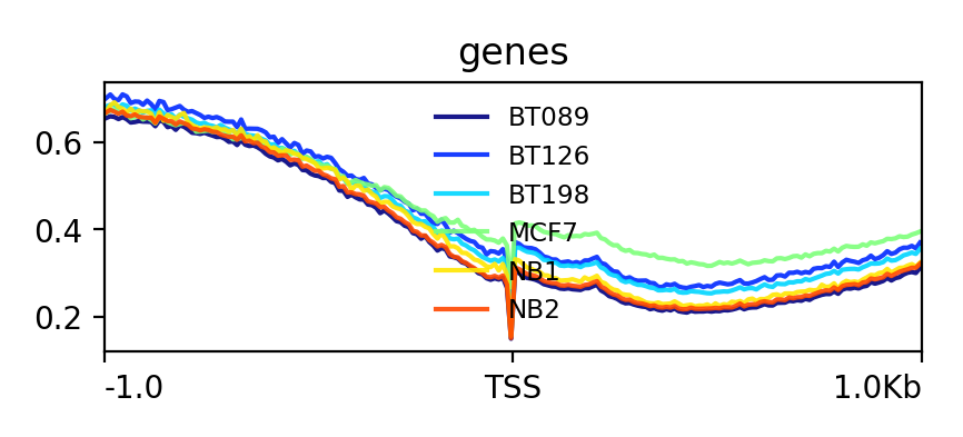
Lets see how the methylation looks for a few provided files:
Import the BED file with CpG islands from Zenodo into the history
https://zenodo.org/records/557099/files/NB1_CpG.meth.bedGraph- Wig/BedGraph-to-bigWig with the following parameters:
- “Convert”:
NB1_CpG.meth.bedGraphQuestionThe execution fails. Do you have an idea why?
A conversion to bigWig would fail right now. If it turned green, the file size should be 0 bytes. Probably dataset info box shows some error message like
hashMustFindVal: '1' not found. The reason is the source of the reference genome which was used. There is ensembl and UCSC as sources which differ in naming the chromosomes. Ensembl is using just numbers e.g. 1 for chromosome one. UCSC is using chr1 for the same. Be careful with this especially if you have data from different sources. We need to convert this.Comment: UCSC - Ensembl convertDownload the file containing mapping between Ensembl and UCS chromosome convention of hg38
https://raw.githubusercontent.com/dpryan79/ChromosomeMappings/master/GRCh38_ensembl2UCSC.txtReplace column ( Galaxy version 0.2) with the follwing parameters:
- “File in which you want to replace some values”:
NB1_CpG.meth.bedGraph- “Replace information file”:
GRCh38_ensembl2UCSC.txt- “Which column should be replaced?”:
Column: 1- “Skip this many starting lines”:
1- “Delimited by”:
TabTo save compute time we prepared the converted files for you. Import the following files. Create a collection list and label it
all_coverage_files. Strip the file extension from the name. For example, rename fromNB1_CpG.meth_ucsc.bedGraphtoNB1_CpG.https://zenodo.org/records/557099/files/NB1_CpG.meth_ucsc.bedGraph https://zenodo.org/records/557099/files/NB2_CpG.meth_ucsc.bedGraph https://zenodo.org/records/557099/files/BT089_CpG.meth_ucsc.bedGraph https://zenodo.org/records/557099/files/BT126_CpG.meth_ucsc.bedGraph https://zenodo.org/records/557099/files/BT198_CpG.meth_ucsc.bedGraph https://zenodo.org/records/557099/files/MCF7_CpG.meth_ucsc.bedgraph
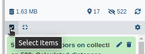
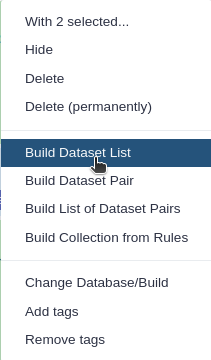
- Click on galaxy-selector Select Items at the top of the history panel
- Check all the datasets in your history you would like to include
Click n of N selected and choose Advanced Build List
You are in collection building wizard. Choose Flat List and click ‘Next’ button at the right bottom corner.
Double clcik on the file names to edit. For example, remove file extensions or common prefix/suffixes to cleanup the names.
- Enter a name for your collection
- Click Build to build your collection
- Click on the checkmark icon at the top of your history again
Change the datatype to
bedgraphand set the database tohg38
- Click on the galaxy-pencil pencil icon for the dataset to edit its attributes
- In the central panel, click galaxy-chart-select-data Datatypes tab on the top
- In the galaxy-chart-select-data Assign Datatype, select
bedgraphfrom “New Type” dropdown
- Tip: you can start typing the datatype into the field to filter the dropdown menu
- Click the Save button
- Click the desired dataset’s name to expand it.
Click on the “?” next to database indicator:
- In the central panel, change the Database/Build field
- Select your desired database key from the dropdown list:
hg38- Click the Save button
- Wig/BedGraph-to-bigWig with the following parameters:
- param-collection “Convert”:
all_coverage_files- computeMatrix ( Galaxy version 3.5.4+galaxy0) with the following parameters:
- “Regions to plot”:
CpGIslands.bed- “Sample order matters”:
No- “Score file”: Output of previous Wig/BedGraph-to-bigWig tool
- “computeMatrix has two main output options”:
reference-point- plotProfile ( Galaxy version 3.5.4+galaxy0) with the following parameters:
- “Matrix file from the computeMatrix tool”:
Matrix(output of previous computeMatrix tool)- “Show advanced options”:
Yes
- “Make one plot per group of regions”: param-toggle
YesThe output should look like this:


Metilene
Hands On: MetileneWith metilene it is possible to detect differentially methylated regions (DMRs) which is a necessary prerequisite for characterizing different epigenetic states.
Import the following files from Zenodo into yout history
https://zenodo.org/records/557099/files/NB1_CpG.meth.bedGraph
https://zenodo.org/records/557099/files/NB2_CpG.meth.bedGraph
https://zenodo.org/records/557099/files/BT198_CpG.meth.bedGraph
Metilene ( Galaxy version 0.2.6.1) with the following parameters:
- “Input group 1”:
NB1_CpG.meth.bedGraphandNB2_CpG.meth.bedGraph- “Input group 2”:
BT198_CpG.meth.bedGraph- “BED file containing regions of interest”:
CpGIslands.bedQuestionHave a look at the produced pdf document. What is the data showing?
It shows the distribution of DMR differences, DMR length in nucleotides and number CpGs, DMR differences vs. q-values, mean methylation group 1 vs. mean methylation group 2 and DMR length in nucleotides vs. length in CpGs
You've Finished the Tutorial
Key points
The output of a methylation NGS is having a different distribution of the four bases. This is caused by the bisulfite treatment of the DNA.
If there is a different level of methylation in the loci of a gene this can be a hint that something is wrong.
To get useful results you need – data, data and data!
Frequently Asked Questions
Have questions about this tutorial? Have a look at the available FAQ pages and support channelsReferences
- Lin, I.-H., D.-T. Chen, Y.-F. Chang, Y.-L. Lee, C.-H. Su et al., 2015 Hierarchical Clustering of Breast Cancer Methylomes Revealed Differentially Methylated and Expressed Breast Cancer Genes (O. El-Maarri, Ed.). PLOS ONE 10: e0118453. 10.1371/journal.pone.0118453
Feedback
Did you use this material as an instructor? Feel free to give us feedback on how it went.
Did you use this material as a learner or student? Click the form below to leave feedback.

Citing this Tutorial
- Joachim Wolff, Devon Ryan, Verena Moosmann, DNA Methylation data analysis (Galaxy Training Materials). https://training.galaxyproject.org/training-material/topics/epigenetics/tutorials/methylation-seq/tutorial.html Online; accessed TODAY
- Hiltemann, Saskia, Rasche, Helena et al., 2023 Galaxy Training: A Powerful Framework for Teaching! PLOS Computational Biology 10.1371/journal.pcbi.1010752
- Batut et al., 2018 Community-Driven Data Analysis Training for Biology Cell Systems 10.1016/j.cels.2018.05.012
Congratulations on successfully completing this tutorial!@misc{epigenetics-methylation-seq, author = "Joachim Wolff and Devon Ryan and Verena Moosmann", title = "DNA Methylation data analysis (Galaxy Training Materials)", year = "", month = "", day = "", url = "\url{https://training.galaxyproject.org/training-material/topics/epigenetics/tutorials/methylation-seq/tutorial.html}", note = "[Online; accessed TODAY]" } @article{Hiltemann_2023, doi = {10.1371/journal.pcbi.1010752}, url = {https://doi.org/10.1371%2Fjournal.pcbi.1010752}, year = 2023, month = {jan}, publisher = {Public Library of Science ({PLoS})}, volume = {19}, number = {1}, pages = {e1010752}, author = {Saskia Hiltemann and Helena Rasche and Simon Gladman and Hans-Rudolf Hotz and Delphine Larivi{\`{e}}re and Daniel Blankenberg and Pratik D. Jagtap and Thomas Wollmann and Anthony Bretaudeau and Nadia Gou{\'{e}} and Timothy J. Griffin and Coline Royaux and Yvan Le Bras and Subina Mehta and Anna Syme and Frederik Coppens and Bert Droesbeke and Nicola Soranzo and Wendi Bacon and Fotis Psomopoulos and Crist{\'{o}}bal Gallardo-Alba and John Davis and Melanie Christine Föll and Matthias Fahrner and Maria A. Doyle and Beatriz Serrano-Solano and Anne Claire Fouilloux and Peter van Heusden and Wolfgang Maier and Dave Clements and Florian Heyl and Björn Grüning and B{\'{e}}r{\'{e}}nice Batut and}, editor = {Francis Ouellette}, title = {Galaxy Training: A powerful framework for teaching!}, journal = {PLoS Comput Biol} }
You can use Ephemeris's
shed-tools installcommand to install the tools used in this tutorial.shed-tools install [-g GALAXY] [-a API_KEY] -t <(curl https://training.galaxyproject.org/training-material/api/topics/epigenetics/tutorials/methylation-seq/tutorial.json | jq .admin_install_yaml -r)Alternatively you can copy and paste the following YAML
---
install_tool_dependencies: true
install_repository_dependencies: true
install_resolver_dependencies: true
tools:
- name: deeptools_compute_matrix
  owner: bgruening
  revisions: fd1275e01605
  tool_panel_section_label: deepTools
  tool_shed_url: https://toolshed.g2.bx.psu.edu/
- name: deeptools_compute_matrix
  owner: bgruening
  revisions: a60c359ec43c
  tool_panel_section_label: deepTools
  tool_shed_url: https://toolshed.g2.bx.psu.edu/
- name: deeptools_plot_profile
  owner: bgruening
  revisions: aac8444d6681
  tool_panel_section_label: deepTools
  tool_shed_url: https://toolshed.g2.bx.psu.edu/
- name: deeptools_plot_profile
  owner: bgruening
  revisions: 6662b1a8d326
  tool_panel_section_label: deepTools
  tool_shed_url: https://toolshed.g2.bx.psu.edu/
- name: pileometh
  owner: bgruening
  revisions: 906db57d5d65
  tool_panel_section_label: Peak Calling
  tool_shed_url: https://toolshed.g2.bx.psu.edu/
- name: pileometh
  owner: bgruening
  revisions: d6787bab7b11
  tool_panel_section_label: Peak Calling
  tool_shed_url: https://toolshed.g2.bx.psu.edu/
- name: replace_column_by_key_value_file
  owner: bgruening
  revisions: cc18bac5afdb
  tool_panel_section_label: Text Manipulation
  tool_shed_url: https://toolshed.g2.bx.psu.edu/
- name: replace_column_by_key_value_file
  owner: bgruening
  revisions: d533e4b75800
  tool_panel_section_label: Text Manipulation
  tool_shed_url: https://toolshed.g2.bx.psu.edu/
- name: text_processing
  owner: bgruening
  revisions: e39fceb6ab85
  tool_panel_section_label: Text Manipulation
  tool_shed_url: https://toolshed.g2.bx.psu.edu/
- name: text_processing
  owner: bgruening
  revisions: d698c222f354
  tool_panel_section_label: Text Manipulation
  tool_shed_url: https://toolshed.g2.bx.psu.edu/
- name: fastqc
  owner: devteam
  revisions: 484e86282f4b
  tool_panel_section_label: FASTA/FASTQ
  tool_shed_url: https://toolshed.g2.bx.psu.edu/
- name: bwameth
  owner: iuc
  revisions: a6ea26c1f225
  tool_panel_section_label: Mapping
  tool_shed_url: https://toolshed.g2.bx.psu.edu/
- name: bwameth
  owner: iuc
  revisions: cf1322aeb137
  tool_panel_section_label: Mapping
  tool_shed_url: https://toolshed.g2.bx.psu.edu/
- name: falco
  owner: iuc
  revisions: 959a14c1f2dd
  tool_panel_section_label: FASTA/FASTQ
  tool_shed_url: https://toolshed.g2.bx.psu.edu/
- name: metilene
  owner: rnateam
  revisions: 37abd09a0ae6
  tool_panel_section_label: Epigenetics
  tool_shed_url: https://toolshed.g2.bx.psu.edu/