RAD-Seq de-novo data analysis
| Author(s) |
|
| Editor(s) |
|
| Reviewers |
|
OverviewQuestions:
Objectives:
How to analyze RAD sequencing data without a reference genome for a population genomics study?
Requirements:
Analysis of RAD sequencing data without a reference genome
SNP calling from RAD sequencing data
Calculate population genomics statistics from RAD sequencing data
Time estimation: 8 hoursSupporting Materials:Published: Feb 14, 2017Last modification: May 7, 2026License: Tutorial Content is licensed under Creative Commons Attribution 4.0 International License. The GTN Framework is licensed under MITpurl PURL: https://gxy.io/GTN:T00128rating Rating: 4.5 (0 recent ratings, 2 all time)version Revision: 15
In the study of Hohenlohe et al. 2010, a genome scan of nucleotide diversity and differentiation in natural populations of threespine stickleback Gasterosteus aculeatus was conducted. Authors used Illumina-sequenced RAD tags to identify and type over 45,000 single nucleotide polymorphisms (SNPs) in each of 100 individuals from two oceanic and three freshwater populations.
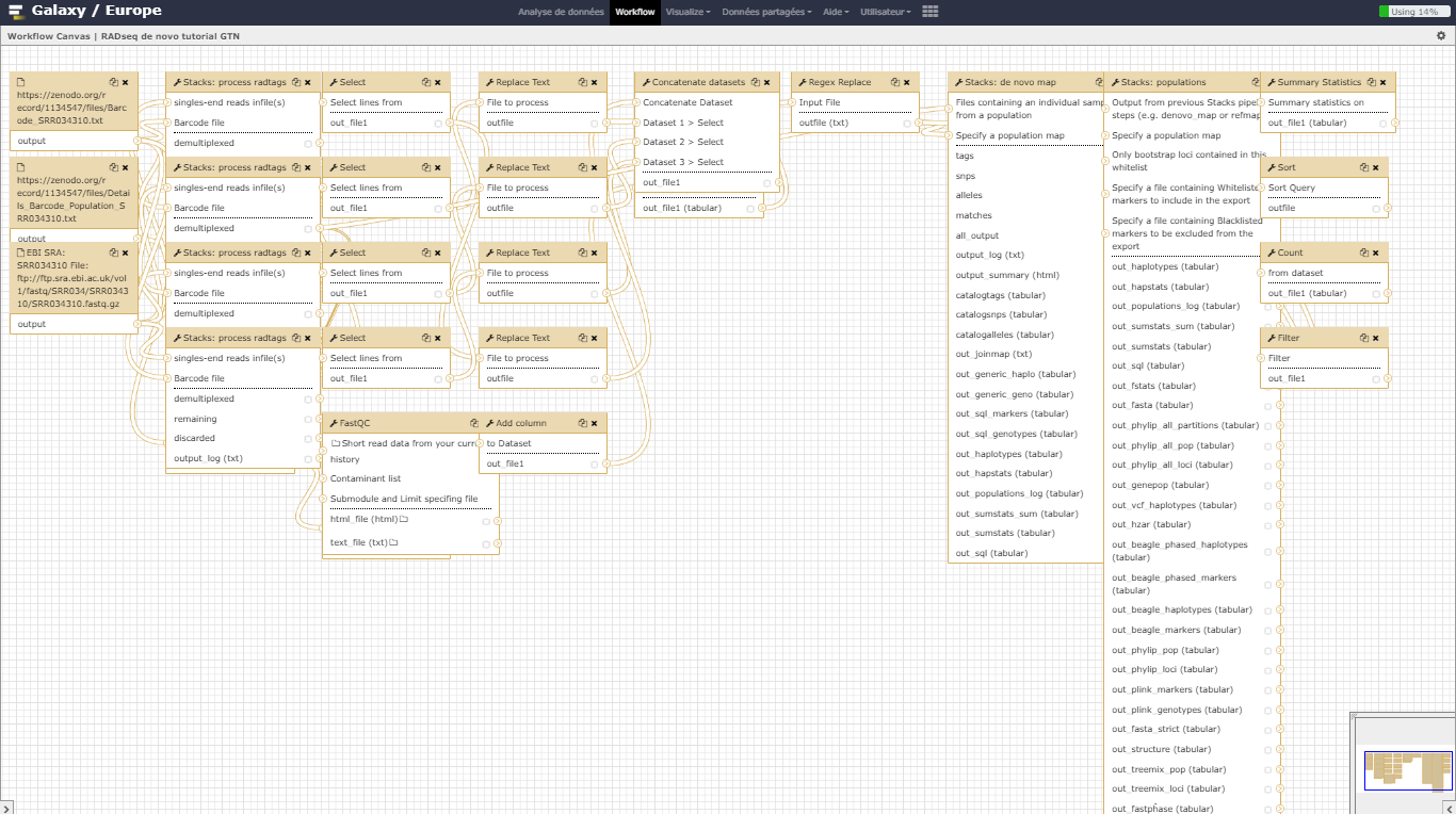
We here proposed to re-analyze these data at least until the population genomics statistics calculation step using STACKS pipeline. Existing Gasterosteus aculeatus draft genome will not be used here so the analysis will be performed de novo. In a de novo RAD-seq data analysis, the reads are aligned one on each other to create stacks and then clustered to build loci. A reference approach can also be conducted (see ref_based tutorial, allowing to work on existing assembled loci).
AgendaIn this tutorial, we will deal with:
Pretreatments
Data upload
The original data is available at NCBI SRA ENA under accession number SRR034310 as part of the NCBI SRA ENA study accession number SRP001747.
We will look at the first run SRR034310 out of seven which includes 16 samples from 2 populations, 8 from Bear Paw (freshwater) and 8 from Rabbit Slough (oceanic). We will download the reads directly from SRA and the remaining data (i.e reference genome, population map file, and barcodes file) from Zenodo.
Hands On: Data upload
Create a new history for this RAD-seq exercise. If you are not inspired, you can name it STACKS RAD: population genomics without reference genome for example…
To create a new history simply click the new-history icon at the top of the history panel:
- EBI SRA tool with the following parameters:
- Select the Run from the results of the search for
SRR034310(which will present you 1 Experiment (SRX015877) and 1 Run (SRR034310)).- Click the link in the column FASTQ files (Galaxy) of the results table
- This will redirect to the Galaxy website and start the download.
- Upload remaining training data from Zenodo:
https://zenodo.org/record/1134547/files/Barcode_SRR034310.txt
https://zenodo.org/record/1134547/files/Details_Barcode_Population_SRR034310.txt
- Copy the link location
Click galaxy-upload Upload at the top of the activity panel
- Select galaxy-wf-edit Paste/Fetch Data
Paste the link(s) into the text field
Press Start
- Close the window
Make sure your fasta files are of datatype
fastqsanger
- Click on the galaxy-pencil pencil icon for the dataset to edit its attributes
- In the central panel, click galaxy-chart-select-data Datatypes tab on the top
- In the galaxy-chart-select-data Assign Datatype, select
fastqsangerfrom “New Type” dropdown
- Tip: you can start typing the datatype into the field to filter the dropdown menu
- Click the Save button


The sequences are raw sequences from the sequencing machine, without any pretreatments. They need to be demultiplexed. To do so, we can use the Process Radtags tool from STACKS.
Demultiplexing reads
For demultiplexing, we use the Process Radtags tool from STACKS .
Hands On: Demultiplexing reads
- Process Radtags tool to demultiplex the reads:
- “Single-end or paired-end reads files”:
Single-end files- “singles-end reads infile(s)”:
SRR034310.fastq(.gz)- “Barcode file”:
Barcodes_SRR034310.tabular- “Number of enzymes”:
One- “Enzyme”:
sbfI- “Capture discarded reads to a file”:
Yes- “Output format:”
fastqQuestion
- How many reads where on the original dataset?
- How many are kept?
- Can you try to explain the reason why we loose a lot of reads here?
- What kind of information does this result give concerning the upcoming data analysis and the barcodes design in general?
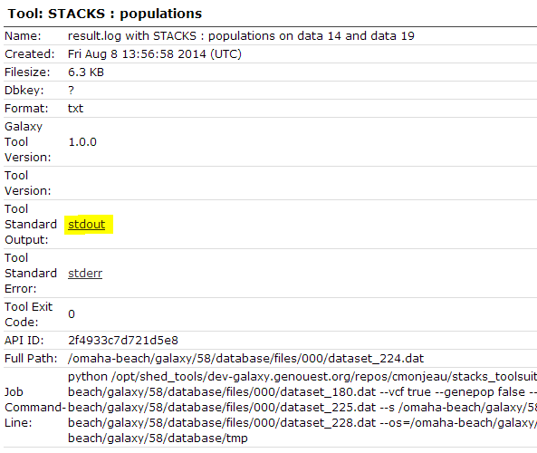
The informations can be found in the results log file:
- 8895289 total reads
- 8139531 retained reads
- There are no sequences filtered because of low quality. This is because radtags didn’t apply quality related filtering since the corresponding advanced option (Discard reads with low quality scores) has not been enabled. So here, all not retained sequences are removed because of an ambiguous barcode (
626265) or an ambiguous RAD-Tag (129493). This means that some barcodes are not exactly what was specified on the barcode file and that sometimes, no SbfI restriction enzyme site was found. This can be due to some sequencing problems but here, this is also due to the addition, in the original sequencing library, of RAD-seq samples from another study. This strategy is often used to avoid having too much sequences beginning with the exact same nucleotide sequence which may cause Illumina related issues during sequencing and cluster analysis- Sequencing quality is essential! Each time your sequencing quality decreases, you loose data and thus essential biological information!
In addition to the overall statistics the numbers of retained and removed reads are also given for each bar code sequence.
Next we will play around with the parameters a bit, to see the impact they have on the results.
- Process Radtags tool: Re-Run playing with parameters
- Section Advanced
- “Discard reads with low quality scores”:
Yes- “score limit”:
20(for example; play with this)- “Set the size of the sliding window as a fraction of the read length, between 0 and 1”:
0.30(for example; play with this)This sliding window parameter allows notably the user to deal with the declining quality at the 3’ end of reads.
Hands OnYou can use the
Chartsfunctionality through the Visualize button reachable on theRadtags logsfile you just generated.If like me you don’t have payed attention to the organization of you file for the graphical representation you obtain a non optimal bars diagram with a not intelligent X-axis ordering. There is a lot of different manner to fix this. You can use a copy/paste “bidouille” or you can use Galaxy tools to manipulate the
radtags logsfile to generate a better graph. For example, you can useSelect lines that match an expressiontool to select rows then use theConcatenate datasets tail-to-headtool to reorganize these lines in a new file. Then we generate a graphical display of the changes:First we cut the interesting lines of each
result.log with Stacks: process radtags
- Select lines that match an expression applying
^R1.fq.gzon the log files and then- Replace Text in entire line on the resulting data sets finding
R1.fq.gzand replacing withNoScoreLimitorScore10orScore20depending of the case- Select lines that match an expression applying
File\tRetained Readson one of the log file to obtain you futur header- Replace Text in entire line on the resulting data set finding
Fileand replacing with#to have a best display- Concatenate datasets tail-to-head on the resulting data sets stating from the header you just created
- Finally Convert delimiters to TAB on the resulting data set converting all Tabs to be sure having a well formatted tabular file at the end
Alternatively just copy/paste these lines on the Galaxy upload tool using Paste/fetch data section and modifying the File header by sample and filename by Score 10 / Score 20 and Lowquality for example… Before Starting the upload, you can select the
Convert spaces to tabsoption through theUpload configurationwheel. If you did not pay attention to the order you can just sort the file using the first column.
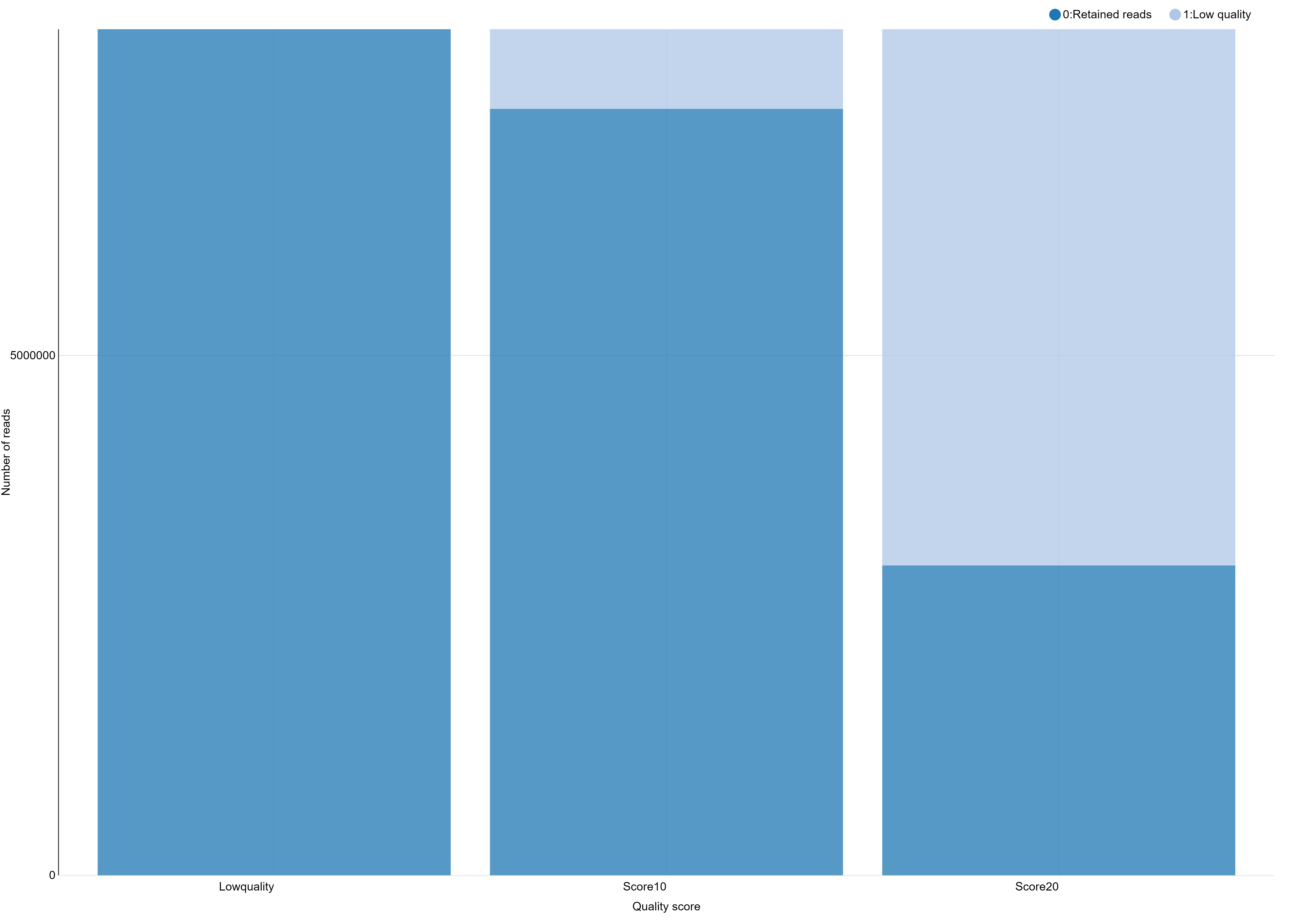
You can use the Charts functionality through the Visualize button to plot the data.
And you obtain a file like this one, ready to generate a beautiful and smart bar stacked!
#		Retained Reads	Low Quality	Ambiguous Barcodes	Ambiguous RAD-Tag	Total
NoScoreLimit	8139531		0		626265			129493			8895289
Score10		7373160		766371		626265			129493			8895289
Score20		2980543		5158988		626265			129493			8895289
You can further test using a filter like clean data, remove any read with an uncalled base and see that here, this has only little impact on the number of retained reads.
The demultiplexed sequences are raw sequences from the sequencing machine, without any pretreatments. They need to be controlled for their quality.
We propose to continue the tutorial using the dataset collection containing the demultiplexed reads obtained with Process Radtag execution made with a quality score of 10 and with the Discard reads with low quality scores parameter set to Yes (so containing 7373160 retained reads).
Quality control
For quality control, we use similar tools as described in NGS-QC tutorial: Falco.
Falco is an efficiency-optimized rewrite of FastQC.
Hands On: Quality control
Falco tool: Run Falco on FastQ files to control the quality of the reads. Warning! Don’t forget you are working on data collections….
Question
- What is the read length?
The read length is 32 bp
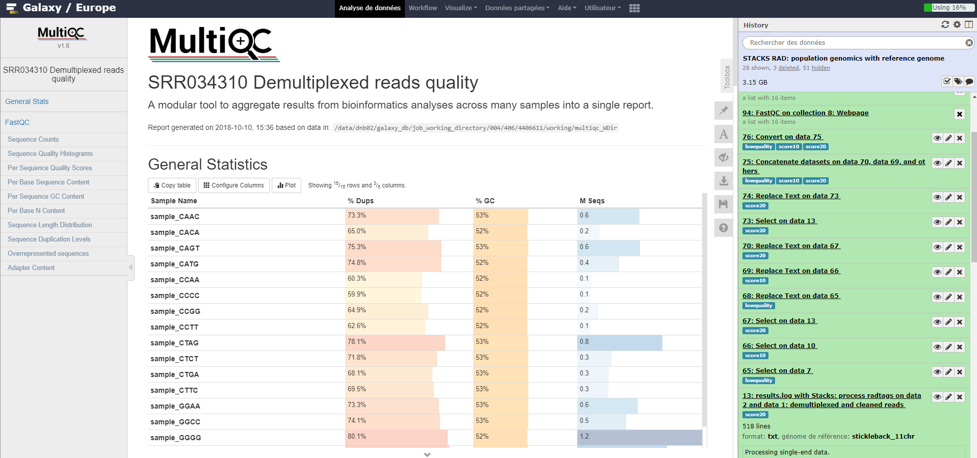
MultiQC tool: Run MultiQC on Falco results to better see quality information over samples. For “Which tool was used generate logs?” choose
FastQCno matter whether FastQC or Falco was used.
SNP calling from radtags
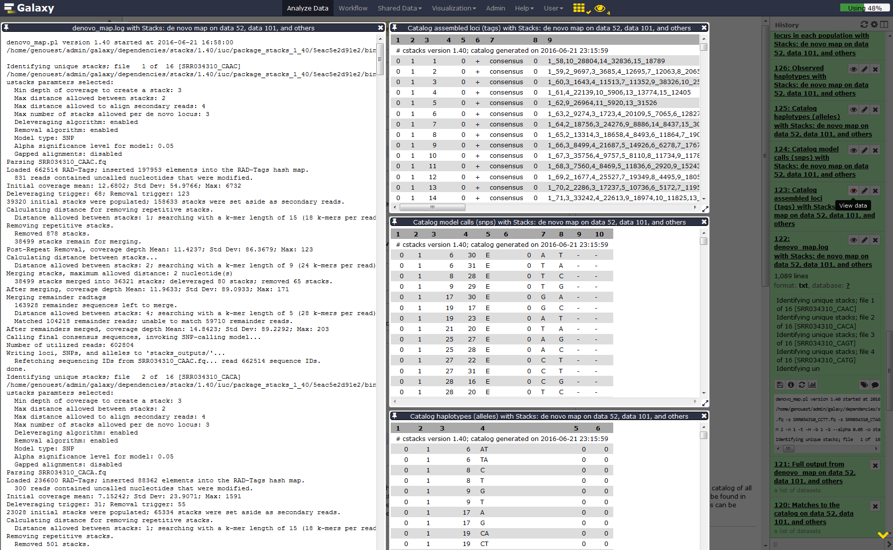
Run Stacks: De novo map Galaxy tool. This program will run ustacks, cstacks, and sstacks on the members of the population, accounting for the alignments of each read.
CommentInformation on denovo_map.pl and its parameters can be found online: https://creskolab.uoregon.edu/stacks/comp/denovo_map.php.
Hands On: Stacks: De novo map
First we will create a population map file with the following contents:
sample_CCCC	1
sample_CCAA	1
sample_CCTT	1
sample_CCGG	1
sample_CACA	1
sample_CAAC	1
sample_CATG	1
sample_CAGT	1
sample_CTCT	2
sample_CTAG	2
sample_CTTC	2
sample_CTGA	2
sample_GGGG	2
sample_GGAA	2
sample_GGTT	2
sample_GGCC	2
- Click galaxy-upload Upload Data at the top of the tool panel
- Select galaxy-wf-edit Paste/Fetch Data at the bottom
- Paste the file contents into the text field
- Press Start and Close the window
- Stacks: De novo map tool: with the following parameters:
- “Select your usage”:
Population- “Files containing an individual sample from a population”:
The demultiplexed reads (collection)- “Specify a population map”:
the population map you just created- Section Assembly options
- “Minimum number of identical raw reads required to create a stack”:
3- “Number of mismatches allowed between loci when building the catalog”:
3- “Remove, or break up, highly repetitive RAD-Tags in the ustacks program”:
YesOnce Stacks has completed running, investigate the output files:
result.logandcatalog.(snps, alleles and tags).
Comment: Data formattingIf you are using a file presenting population information and individual name in a different manner than expected by STACKS, you can use Galaxy tools like
Replace Text(for example to replaceRabbit Sloughby a population number like2,Add column(for example to addsample_) orCut columns from a table(to put the newsample_column af the first place) and finallyRegex replace(replacing(sample_)\tby\1) to generate it…
Calculate population genomics statistics
Hands On: Calculate population genomics statistics
- Stacks: populations tool with the following parameters:
- Section Data filtering options
- “Minimum percentage of individuals in a population required to process a locus for that population”:
0.75- Section Output options (VCF and Structure) and enabling SNP and haplotype-based F statistics calculation.
- “Output results in Variant Call Format (VCF)”:
Yes- “Output results in Structure Format”:
Yes- “Enable SNP and haplotype-based F statistics”:
Yes
- Now look at the output in the file
batch_1.sumstatsnammedSNP and Haplotype-based F statistics with Stacks: populations ...on your history. There are a large number of statistics calculated at each SNP, so use Galaxy tools like filter, cut, and sort to focus on some.Question
- What is the maximum value of FST’ at any SNP? Don’t hesitate to look at the STACKS manual to find where this parameter is
- What is the meaning of this FST’ value compared a a classical FST one? Once again, the STACKS manual can help you ;)
- How many SNPs reach this FST’ value?
- 1
- FST’ is a haplotype measure of FST that is scaled to the theoretical maximum FST value at this locus. Depending on how many haplotypes there are, it may not be possible to reach an FST of 1, so this method will scale the value to 1
- 114
You can now for example filter this dataset to only keep FST’=1 loci for further analysis…
Conclusion
In this tutorial, we have analyzed real RAD sequencing data to extract useful information, such as which loci are candidate regarding the genetic differentiation between freshwater and oceanic Stickelback populations. To answer these questions, we analyzed RAD sequence datasets using a de novo RAD-seq data analysis approach. This approach can be sum up with the following scheme:
You've Finished the Tutorial
Frequently Asked Questions
Have questions about this tutorial? Have a look at the available FAQ pages and support channelsUseful literature
Further information, including links to documentation and original publications, regarding the tools, analysis techniques and the interpretation of results described in this tutorial can be found here.
Feedback
Did you use this material as an instructor? Feel free to give us feedback on how it went.
Did you use this material as a learner or student? Click the form below to leave feedback.

Citing this Tutorial
- Yvan Le Bras, RAD-Seq de-novo data analysis (Galaxy Training Materials). https://training.galaxyproject.org/training-material/topics/ecology/tutorials/de-novo-rad-seq/tutorial.html Online; accessed TODAY
- Hiltemann, Saskia, Rasche, Helena et al., 2023 Galaxy Training: A Powerful Framework for Teaching! PLOS Computational Biology 10.1371/journal.pcbi.1010752
- Batut et al., 2018 Community-Driven Data Analysis Training for Biology Cell Systems 10.1016/j.cels.2018.05.012
Congratulations on successfully completing this tutorial!@misc{ecology-de-novo-rad-seq, author = "Yvan Le Bras", title = "RAD-Seq de-novo data analysis (Galaxy Training Materials)", year = "", month = "", day = "", url = "\url{https://training.galaxyproject.org/training-material/topics/ecology/tutorials/de-novo-rad-seq/tutorial.html}", note = "[Online; accessed TODAY]" } @article{Hiltemann_2023, doi = {10.1371/journal.pcbi.1010752}, url = {https://doi.org/10.1371%2Fjournal.pcbi.1010752}, year = 2023, month = {jan}, publisher = {Public Library of Science ({PLoS})}, volume = {19}, number = {1}, pages = {e1010752}, author = {Saskia Hiltemann and Helena Rasche and Simon Gladman and Hans-Rudolf Hotz and Delphine Larivi{\`{e}}re and Daniel Blankenberg and Pratik D. Jagtap and Thomas Wollmann and Anthony Bretaudeau and Nadia Gou{\'{e}} and Timothy J. Griffin and Coline Royaux and Yvan Le Bras and Subina Mehta and Anna Syme and Frederik Coppens and Bert Droesbeke and Nicola Soranzo and Wendi Bacon and Fotis Psomopoulos and Crist{\'{o}}bal Gallardo-Alba and John Davis and Melanie Christine Föll and Matthias Fahrner and Maria A. Doyle and Beatriz Serrano-Solano and Anne Claire Fouilloux and Peter van Heusden and Wolfgang Maier and Dave Clements and Florian Heyl and Björn Grüning and B{\'{e}}r{\'{e}}nice Batut and}, editor = {Francis Ouellette}, title = {Galaxy Training: A powerful framework for teaching!}, journal = {PLoS Comput Biol} }
You can use Ephemeris's
shed-tools installcommand to install the tools used in this tutorial.shed-tools install [-g GALAXY] [-a API_KEY] -t <(curl https://training.galaxyproject.org/training-material/api/topics/ecology/tutorials/de-novo-rad-seq/tutorial.json | jq .admin_install_yaml -r)Alternatively you can copy and paste the following YAML
---
install_tool_dependencies: true
install_repository_dependencies: true
install_resolver_dependencies: true
tools:
- name: fastqc
  owner: devteam
  revisions: f2e8552cf1d0
  tool_panel_section_label: FASTA/FASTQ
  tool_shed_url: https://toolshed.g2.bx.psu.edu/
- name: stacks_denovomap
  owner: iuc
  revisions: fdbcc560c691
  tool_panel_section_label: RAD-seq
  tool_shed_url: https://toolshed.g2.bx.psu.edu/
- name: stacks_populations
  owner: iuc
  revisions: 45db1ba16163
  tool_panel_section_label: RAD-seq
  tool_shed_url: https://toolshed.g2.bx.psu.edu/
- name: stacks_procrad
  owner: iuc
  revisions: eded025438db
  tool_panel_section_label: RAD-seq
  tool_shed_url: https://toolshed.g2.bx.psu.edu/