This tutorial will guide you on the exploration of biodiversity data having taxonomic, spatial and temporal informations.

We’ll be using Reef Life Survey (RLS) data extracted from the Australian Ocean Data Network (AODN) portal. We’ll use a subset done directly on the AODN data portal (https://portal.aodn.org.au/) on this dataset “IMOS - National Reef Monitoring Network Sub-Facility - Global reef fish abundance and biomass”. We decided to use data only on the Mollusca phylum from the east coast of Australia between 2008 and 2021. We’ll explore this dataset in the view of making statistical analyses so we will check the homoscedasticity and normality of the variables, see if some variables are correlated, how the data is distributed through space and time, etc … And finally, we’ll explore Beta diversity through the computation of the SCBD and LCBD (Species and Local Contribution to Beta Diversity).

Details: Definitions of SCBD and LCBD

Species Contribution to Beta Diversity: degree of variation for individual species across the study area.

Local Contribution to Beta Diversity: comparative indicators of the ecological uniqueness of the sites.

Agenda

In this tutorial, we will cover:

1. Data preparation
   1. Get data
   2. Customize your dataset
2. Data checking
   1. Homoscedasticity and normality analysis
   2. Autocorrelation in your data
   3. Check collinearity in your data
3. Data exploration
   1. Visualize abundance repartition through space
   2. Visualize the number of locations where each taxons are present
   3. Visualize the rarefaction curves of your species
   4. Visualize the dispersion of a numeric variable and the correlation between species absence
4. Beta diversity
   1. Local and Species Contribution to Beta Diversity (SCBD and LCBD)
5. Conclusion
6. Bonus: Want to spatially anoymize your data?
   1. Bonus! Spatial coordinates anonymization

Data preparation

First step is to download biodiversity data on your Galaxy history. Here we will use a “classical” (containing taxonomic, spatial and temporal informations) biodiversity dataset from the well known “Reef life survey” initiative.

Get data

Hands-on: Data upload

1. Create a new history for this tutorial and give it a name (example: “RLS for biodiversity data exploration tutorial”) for you to find it again later if needed.

2. Import the files from Zenodo

   Tip: Importing via links

   • Copy the link location

   • Click galaxy-upload Upload Data at the top of the tool panel

   • Select galaxy-wf-edit Paste/Fetch Data

   • Paste the link(s) into the text field

   • Press Start

   • Close the window

   Tip: Importing data from a data library

   As an alternative to uploading the data from a URL or your computer, the files may also have been made available from a shared data library:

   1. Go into Data (top panel) then Data libraries
   2. Navigate to the correct folder as indicated by your instructor.
      • On most Galaxies tutorial data will be provided in a folder named GTN - Material –> Topic Name -> Tutorial Name.
   3. Select the desired files
   4. Click on Add to History galaxy-dropdown near the top and select as Datasets from the dropdown menu

   5. In the pop-up window, choose

      • “Select history”: the history you want to import the data to (or create a new one)
   6. Click on Import

3. Rename the datasets “reef_life_molluscs” for example and preview your dataset

   You can see that the dataset hasn’t been detected to be a CSV dataframe, it is because RLS data directly puts the metadata of the dataframe in the first lines before the dataframe so you’ll have to remove these lines using the Remove beginning with the following parameters: - param-text “Remove first”: 72 - param-file “from”: reef_life_molluscs data file

   Then, verify if your new file hasn’t got hashtags in the first lines and then ask Galaxy to autodetect datatype (click on the pencil, then “Datatypes” then click on “Auto-detect” button). Galaxy will normally detect it as csv.

4. Convert datatype CSV to tabular

   Tip: Converting the file format

   • Click on the galaxy-pencil pencil icon for the dataset to edit its attributes
   • In the central panel, click on the galaxy-gear Convert tab on the top
   • In the upper part galaxy-gear Convert, select Convert CSV to tabular
   • Click the Create dataset button to start the conversion.

Customize your dataset

In order to clean unnecessary informations from the table we will now cut a few columns and change the format of time information.

Hands-on: Clean your data

1. Use Advanced cut columns from a table (cut) ( Galaxy version 1.1.0) with following parameters :
   • param-files “File to cut”: Convert CSV to tabular data file
   • param-select “Operation”: Keep
   • param-select “Delimited by”: Tab
   • param-select “Cut by”: fields
     • param-select “List of Fields”: Column: 8 Column: 10 Column: 11 Column: 12 Column: 25 Column: 28
2. Use Column Regex Find And Replace ( Galaxy version 1.0.0) with following parameters:
   • param-files “Select cells from”: Advanced Cut data file
   • param-select “using column”: Column: 4
   • param-repeat Click ”+ Insert Check”:
     • param-text “Find Regex”: ([0-9]{4})-[0-9]{2}-[0-9]{2}
     • param-text “Replacement”: \1

Data checking

Homoscedasticity and normality analysis

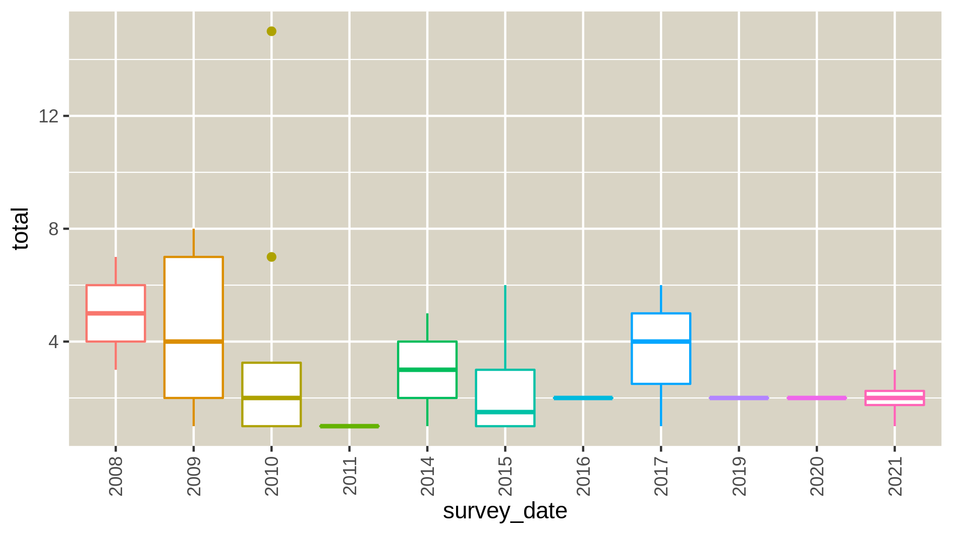
Hands-on: Here we will check homogeneity of variances (Levene test) for every species and represent it through multiple boxplots and the normal distribution (Kolmogorov-Smirnov test) represented by a distribution histogram and a Q-Q plot.

1. Homoscedasticity and normality ( Galaxy version 0.0.0) with the following parameters:
   • param-file “Input table”: Column Regex Find and Replace data file
   • param-select “First line is a header line”: Yes
   • param-select “Select column containing temporal data (year, date, …)”: c4
   • param-select “Select column containing species”: c5
   • param-select “Select column containing numerical values (like abundances)”: c6

   You have to get three outputs: the Levene Test for homoscedasticity dataset, the Kolmogrov-Smirnov test for normality and 9 PNG files in a data collection representing the homogeneity of variances for each species at each time point of the study. If the levene test is significant (P-value in column Pr < 0.5 and at least one * at the end of the 4th line), variances aren’t homogeneous, the hypothesis of homoscedasticity is rejected. If the K-S test is significant (p-value < 0.5), your numerical variable isn’t normally distributed, the hypothesis of normality is rejected. The two tests have to be significant so variances aren’t homogenous and data isn’t normally distributed.

Autocorrelation in your data

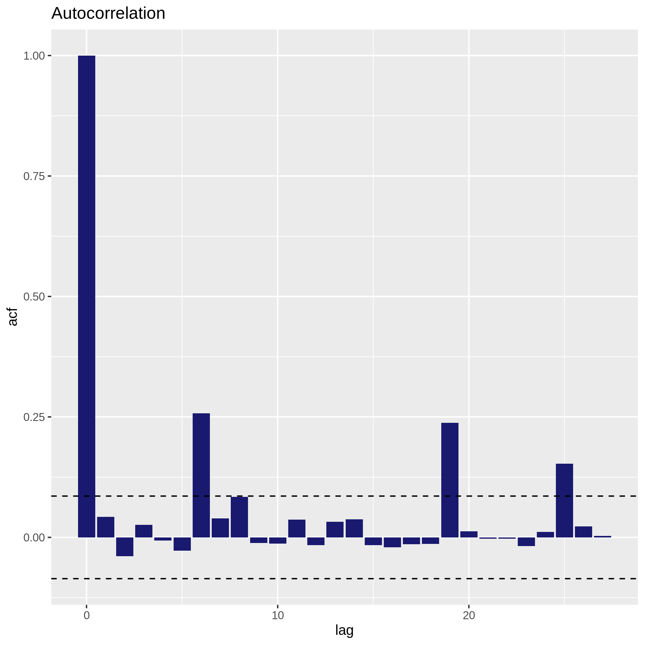
Hands-on: Autocorrelation

1. Variables exploration ( Galaxy version 0.0.0) with the following parameters:
   • param-file “Input table”: Column Regex Find and Replace data file
   • param-select “First line is a header line”: Yes
   • param-select “Variables links exploration”: Autocorrelation of one selected numerical variable
     • param-select “Select columns containing numerical values”: c6

   You have to get two outputs, one text file containing the Autocorrelation function values and one PNG file in the data collection showing the autocorrelation for a variable. If the bars of the histogram are strictly confined between the dashed lines (representing 95% confidence interval without white noise), there is auto-correlation.

   Here, we don’t see there is autocorrelation.

Check collinearity in your data

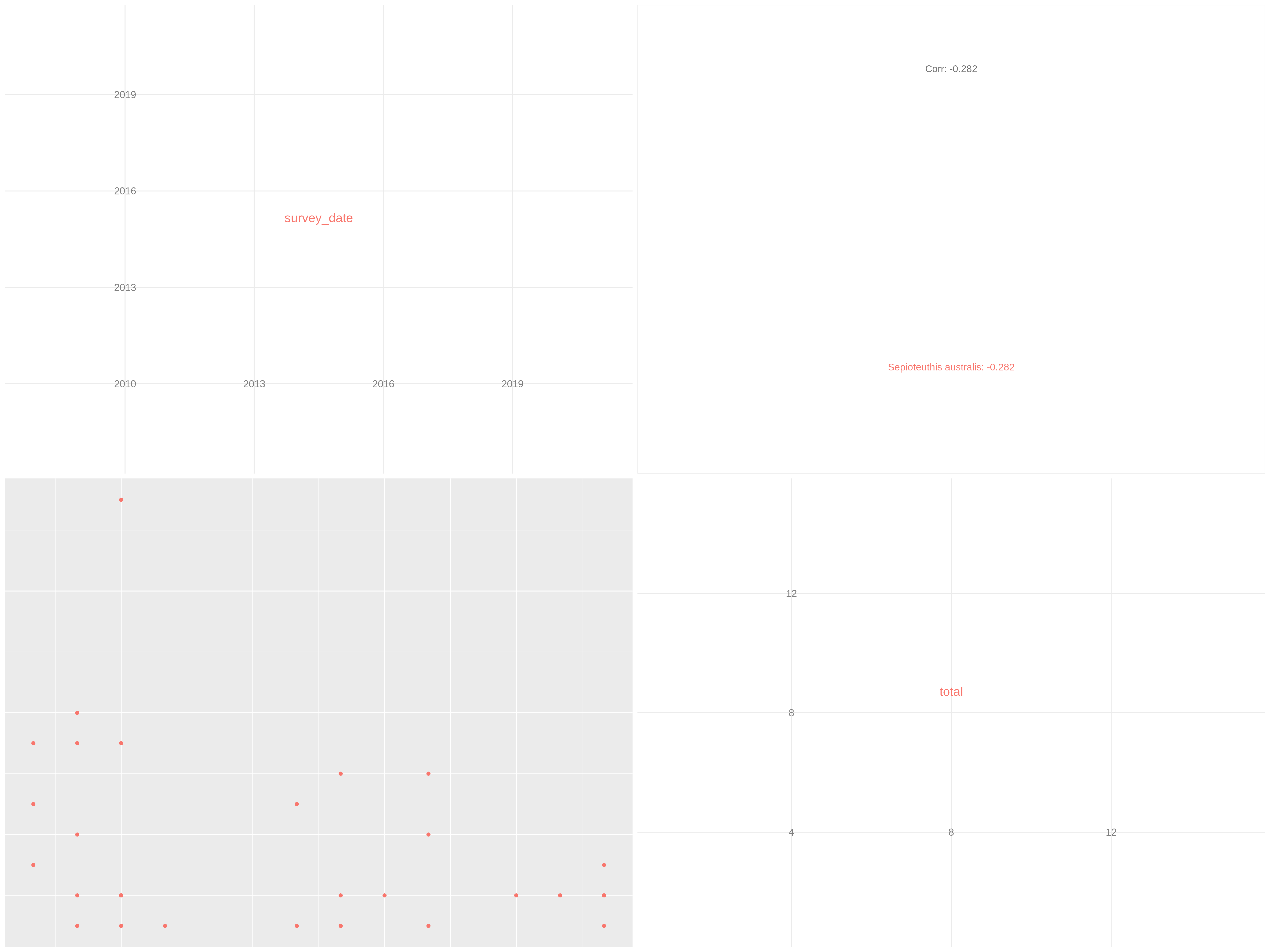
Hands-on: Collinearity between numerical variables

1. Variables exploration ( Galaxy version 0.0.0) with the following parameters:
   • param-file “Input table”: formatted biodiversity data file
   • param-select “First line is a header line”: Yes
   • param-select “Variables links exploration”: Collinearity between selected numerical variables for each species
     • param-select “Select column containing species”: c5
     • param-select “Select columns containing numerical values”: c['4', '6']

   You have to get two outputs, one describing species we couldn’t evaluate and one PNG file with one plot containing multiple correlation plots and the correlation values between each variables.

Data exploration

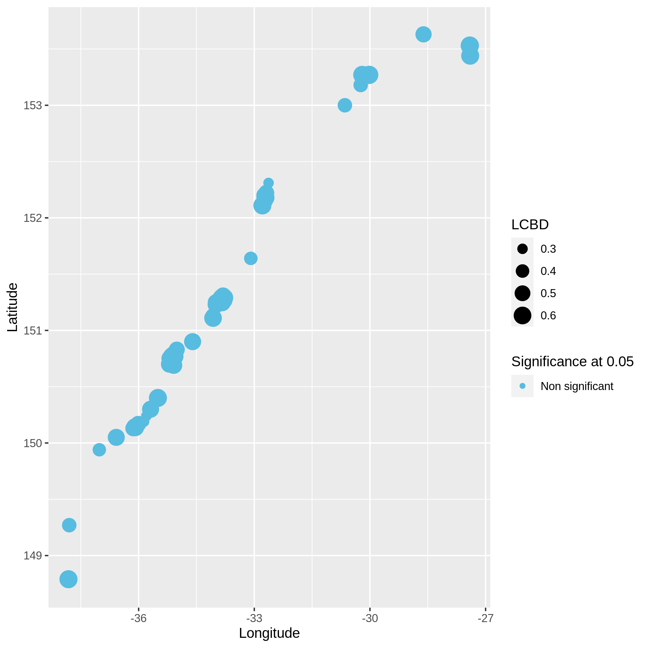
Visualize abundance repartition through space

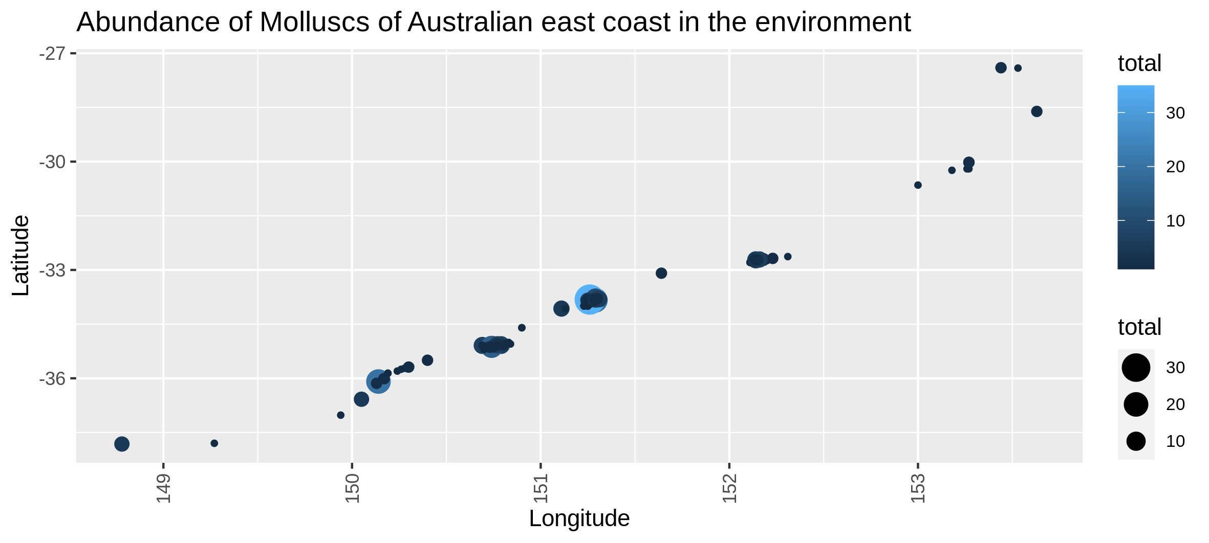
Hands-on: Abundance map in the environment

1. Presence-absence and abundance ( Galaxy version 0.0.0) with the following parameters:
   • param-file “Input table”: formatted biodiversity data file
   • param-select “First line is a header line”: Yes
   • param-select “Variables presence, absence and abundance”: Abundance map in the environment
     • param-select “Select column containing latitudes “: c2
     • param-select “Select column containing longitudes”: c3
     • param-text “What do you study in this analysis ?”: Molluscs of Australian east coast
     • param-select “Select column containing taxon “: c5
   • param-select “Select column containing abundances “: c6

   You have to get two outputs, one with the map of the abundance through space with the coordinates and one text file to inform you about the geographical extent of your map.

Visualize the number of locations where each taxons are present

Hands-on: Presence count of taxons (barplot)

1. Presence-absence and abundance ( Galaxy version 0.0.0) with the following parameters:
   • param-file “Input table”: formatted biodiversity data file
   • param-select “First line is a header line”: Yes
   • param-select “Variables presence, absence and abundance”: Presence count of taxons (barplot)
     • param-select “Select column containing your separation variable”: c1
     • param-select “Select column containing taxon”: c5
   • param-select “Select column containing abundances “: c6

   You have to get two outputs, one with 120 PNG files (one for each site) representing the number of locations where each taxons are present and one text file to inform you about the used locations.

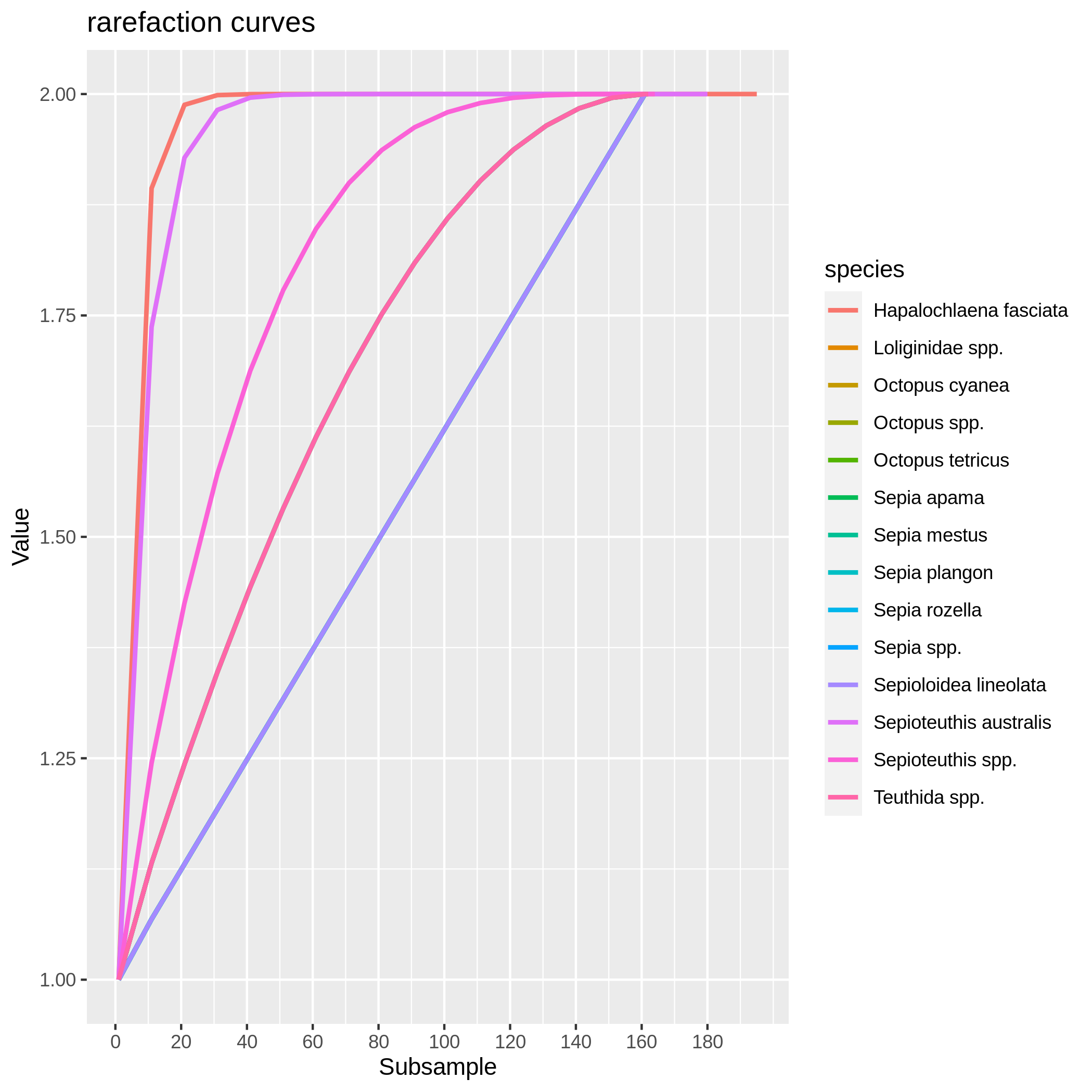
Visualize the rarefaction curves of your species

Hands-on: Rarefaction curve of species

1. Presence-absence and abundance ( Galaxy version 0.0.0) with the following parameters:
   • param-file “Input table”: formatted biodiversity data file
   • param-select “First line is a header line”: Yes
   • param-select “Variables presence, absence and abundance”: Rarefaction curve of species
     • param-text “Size of subsamples”: 200
     • param-select “Select column containing species”: c5
   • param-select “Select column containing abundances “: c6

   You have to get two outputs, one data collection with one PNG files representing the rarefaction curves of each species in one graph and one tabular file with log informations.

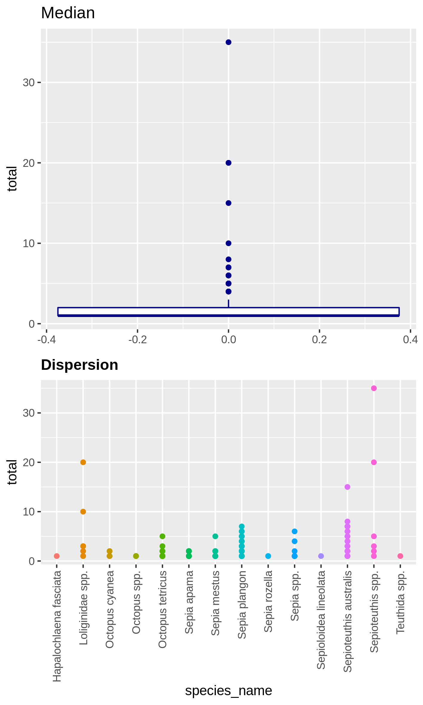
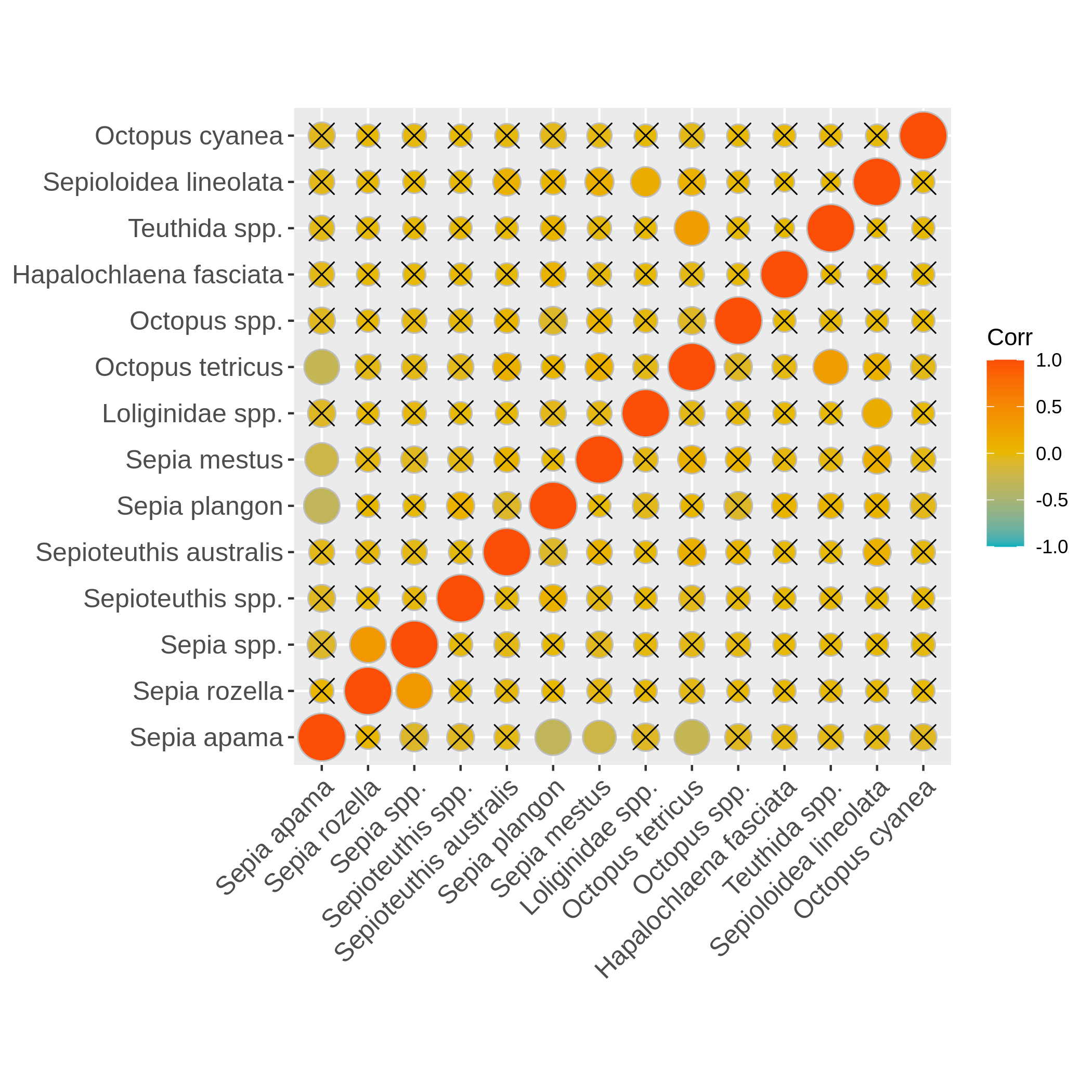
Visualize the dispersion of a numeric variable and the correlation between species absence

Hands-on: Boxplot of dispersion and correlation of absence

1. Statistics on presence-absence ( Galaxy version 0.0.0) with the following parameters:
   • param-file “Input table”: formatted biodiversity data file
   • param-select “First line is a header line”: Yes
   • param-select “Select a column containing numerical values (such as the abundance) “: c6
   • param-select “Select the column of the x-axis : most commonly species”: c5
   • param-select “Select column containing locations “: c1
   • param-select “Select column containing temporal data (year, date, …) “: c4

   You have to get two outputs, one PNG file with the boxplot and dispersion plot of the abundance and one plot representing wether the absence of several species is correlated. In the second plot if you see there is a cross on the round representation the two related species haven’t got their absences correlated, the other are correlated and seem to be co-absent.

Beta diversity

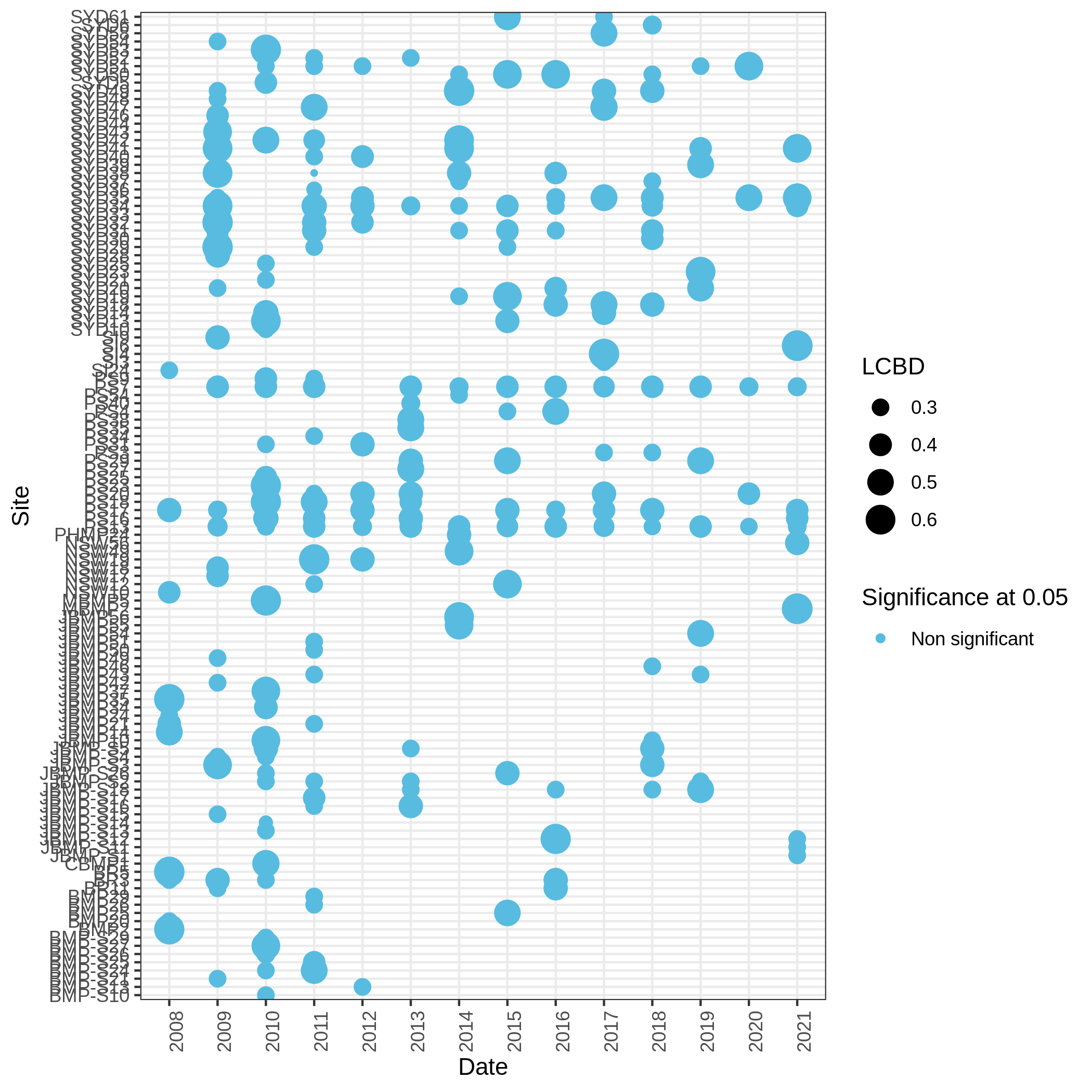
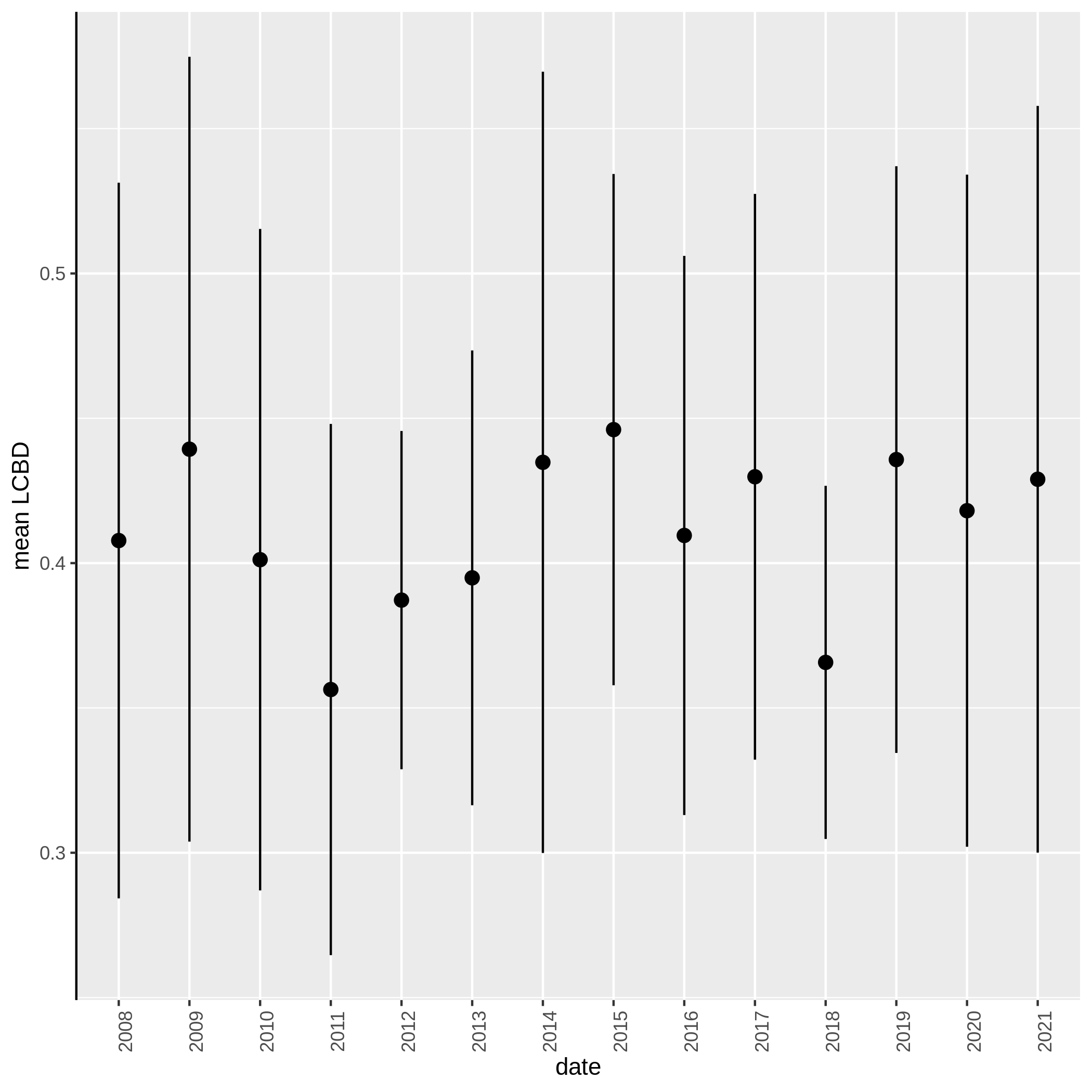
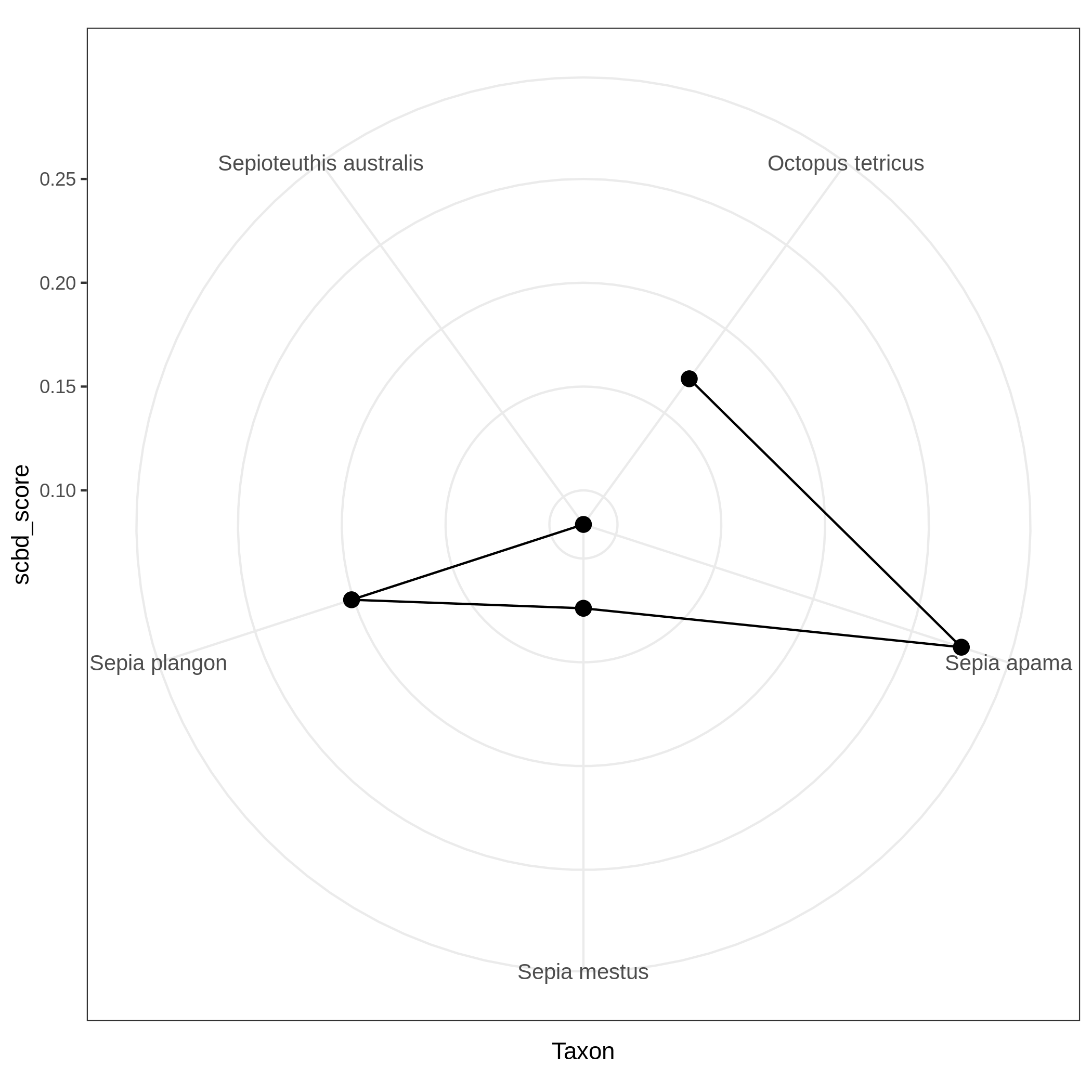
Local and Species Contribution to Beta Diversity (SCBD and LCBD)

Hands-on: Task description

1. Local Contributions to Beta Diversity (LCBD) ( Galaxy version 0.0.0) with the following parameters:
   • param-file “Input table”: formatted biodiversity data file
   • param-select “First line is a header line”: Yes
   • param-select “Select column with abundances”: c6
   • param-select “Select column with locations”: c1
   • param-select “Select column containing taxon”: c5
   • param-select “Select column containing dates”: c4
   • param-select “Other LCBD : spatialized representation or xy plot.”: Spatialized representation
     • param-select “Select column containing latitudes in decimal degrees”: c2
     • param-select “Select column containing longitudes in decimal degrees”: c3

   You have to get three outputs. Two text file containing a table with information on the beta diversity and one text file with the list of species that has a SCBD larger than the mean SCBD. One data collection with PNG files showing multiple plots according to one type of variable in order to vizualize the beta diversity.

Conclusion

Here, you just explored your biodiversity dataframe properly and you know a lot more about your data. You can now peacefully make your statiscal analyses as most of the red flags you can get have been revealed by this toolsuite ! Enjoy !

Bonus: Want to spatially anoymize your data?

A step of this tutorial could be to show you how you can simply apply spatial coordinates anonymization if you want to share data without spatial context, particularly of interest if you want to share endangered species oriented data.

Bonus! Spatial coordinates anonymization

Hands-on: Task description

1. Spatial coordinates anonymization ( Galaxy version 0.0.0) with the following parameters:
   • param-file “Input table”: Column Regex Find and Replace data file
   • param-select “First line is a header line”: Yes
   • param-select “Select column containing latitudes in decimal degrees”: c2
   • param-select “Select column containing longitudes in decimal degrees”: c3

You've Finished the Tutorial

Please also consider filling out the Feedback Form as well!

Key points

• Explore your data before diving into deep analysis

Frequently Asked Questions

Useful literature

Further information, including links to documentation and original publications, regarding the tools, analysis techniques and the interpretation of results described in this tutorial can be found here.

Feedback

Did you use this material as an instructor? Feel free to give us feedback on how it went.
Did you use this material as a learner or student? Click the form below to leave feedback.

Citing this Tutorial

1. Olivier Norvez, Marie Josse, Coline Royaux, Yvan Le Bras, Biodiversity data exploration (Galaxy Training Materials). https://training.galaxyproject.org/training-material/topics/ecology/tutorials/biodiversity-data-exploration/tutorial.html Online; accessed TODAY
2. Hiltemann, Saskia, Rasche, Helena et al., 2023 Galaxy Training: A Powerful Framework for Teaching! PLOS Computational Biology 10.1371/journal.pcbi.1010752
3. Batut et al., 2018 Community-Driven Data Analysis Training for Biology Cell Systems 10.1016/j.cels.2018.05.012

BibTeX

@misc{ecology-biodiversity-data-exploration,
author = "Olivier Norvez and Marie Josse and Coline Royaux and Yvan Le Bras",
	title = "Biodiversity data exploration (Galaxy Training Materials)",
	year = "",
	month = "",
	day = "",
	url = "\url{https://training.galaxyproject.org/training-material/topics/ecology/tutorials/biodiversity-data-exploration/tutorial.html}",
	note = "[Online; accessed TODAY]"
}
@article{Hiltemann_2023,
	doi = {10.1371/journal.pcbi.1010752},
	url = {https://doi.org/10.1371%2Fjournal.pcbi.1010752},
	year = 2023,
	month = {jan},
	publisher = {Public Library of Science ({PLoS})},
	volume = {19},
	number = {1},
	pages = {e1010752},
	author = {Saskia Hiltemann and Helena Rasche and Simon Gladman and Hans-Rudolf Hotz and Delphine Larivi{\`{e}}re and Daniel Blankenberg and Pratik D. Jagtap and Thomas Wollmann and Anthony Bretaudeau and Nadia Gou{\'{e}} and Timothy J. Griffin and Coline Royaux and Yvan Le Bras and Subina Mehta and Anna Syme and Frederik Coppens and Bert Droesbeke and Nicola Soranzo and Wendi Bacon and Fotis Psomopoulos and Crist{\'{o}}bal Gallardo-Alba and John Davis and Melanie Christine Föll and Matthias Fahrner and Maria A. Doyle and Beatriz Serrano-Solano and Anne Claire Fouilloux and Peter van Heusden and Wolfgang Maier and Dave Clements and Florian Heyl and Björn Grüning and B{\'{e}}r{\'{e}}nice Batut and},
	editor = {Francis Ouellette},
	title = {Galaxy Training: A powerful framework for teaching!},
	journal = {PLoS Comput Biol}
}

                   

Funding

These individuals or organisations provided funding support for the development of this resource

PNDB

Gallantries

This project (2020-1-NL01-KA203-064717) is funded with the support of the Erasmus+ programme of the European Union. Their funding has supported a large number of tutorials within the GTN across a wide array of topics.

PNDB

FNSO

This project (AAPFNSO2019OpenMetaPaper-14026) is funded with the support of the national Fund for Open Science programme of the French Minister of Higher Education, Research and Innovation. Their funding has supported development of data/metadata management tools and related tutorial for Ecology and FAIR topics.

Galaxy Administrators: Install the missing tools

You can use Ephemeris's shed-tools install command to install the tools used in this tutorial.

shed-tools install [-g GALAXY] [-a API_KEY] -t <(curl https://training.galaxyproject.org/training-material/api/topics/ecology/tutorials/biodiversity-data-exploration/tutorial.json | jq .admin_install_yaml -r)

Alternatively you can copy and paste the following YAML

---
install_tool_dependencies: true
install_repository_dependencies: true
install_resolver_dependencies: true
tools:
- name: text_processing
  owner: bgruening
  revisions: d698c222f354
  tool_panel_section_label: Text Manipulation
  tool_shed_url: https://toolshed.g2.bx.psu.edu/
- name: ecology_beta_diversity
  owner: ecology
  revisions: fb7b2cbd80bb
  tool_panel_section_label: Biodiversity data exploration
  tool_shed_url: https://toolshed.g2.bx.psu.edu/
- name: ecology_homogeneity_normality
  owner: ecology
  revisions: 3df8937fd6fd
  tool_panel_section_label: Biodiversity data exploration
  tool_shed_url: https://toolshed.g2.bx.psu.edu/
- name: ecology_link_between_var
  owner: ecology
  revisions: 8e8867bf491a
  tool_panel_section_label: Biodiversity data exploration
  tool_shed_url: https://toolshed.g2.bx.psu.edu/
- name: ecology_presence_abs_abund
  owner: ecology
  revisions: 4ed07d2d442b
  tool_panel_section_label: Biodiversity data exploration
  tool_shed_url: https://toolshed.g2.bx.psu.edu/
- name: ecology_stat_presence_abs
  owner: ecology
  revisions: 9a2e0195bb43
  tool_panel_section_label: Biodiversity data exploration
  tool_shed_url: https://toolshed.g2.bx.psu.edu/
- name: tool_anonymization
  owner: ecology
  revisions: 726a387cfdc2
  tool_panel_section_label: Biodiversity data exploration
  tool_shed_url: https://toolshed.g2.bx.psu.edu/
- name: regex_find_replace
  owner: galaxyp
  revisions: 209b7c5ee9d7
  tool_panel_section_label: Text Manipulation
  tool_shed_url: https://toolshed.g2.bx.psu.edu/

Feedback

No feedback has been recieved yet for this training. Be the first one by filling in the feedback form from above.