Introduction

What is genome assembly?

Genome assembly is the process of joining together DNA sequencing fragments into longer pieces, ideally up to chromosome lengths.The DNA fragments are produced by DNA sequencing machines, and are called “reads”. These are in lengths of about 150 nucleotides (base pairs), to up to a million+ nucleotides, depending on the sequencing technology used. Currently, most reads are from Illumina (short), PacBio (long) or Oxford Nanopore (long and extra-long).

It is difficult to assemble plant genomes as they are often large (for example, 3,000,000,000 base pairs), have many repeat regions (such as transposons), and may be polyploid. This tutorial shows genome assembly for a smaller data set - the plant chloroplast genome - a single circular chromosome which is typically about 160,000 base pairs. It is thought that the the chloroplast evolved from a cyanobacteria that was living in plant cells.

In this tutorial, we will use a subset of a real data set from sweet potato, from the paper Zhou et al. 2018. To find out more about each of the tools used here, see the tool panel page for a summary and links to more information.

Agenda

In this tutorial we will deal with:

1. Introduction
   1. What is genome assembly?
2. Upload data
3. Check read quality
4. Assemble reads
5. Polish assembly
6. Annotate the assembly
7. View reads
8. Repeat with new data
9. Conclusion

Upload data

Let’s start with uploading the data.

Hands-on: Import the data

1. Create a new history for this tutorial and give it a proper name

   Tip: Creating a new history

   Click the new-history icon at the top of the history panel:

   

   Tip: Renaming a history

   1. Click on galaxy-pencil (Edit) next to the history name (which by default is “Unnamed history”)
   2. Type the new name
   3. Click on Save

   If you do not have the galaxy-pencil (Edit) next to the history name:

   1. Click on Unnamed history (or the current name of the history) (Click to rename history) at the top of your history panel
   2. Type the new name
   3. Press Enter

2. Import from Zenodo or a data library (ask your instructor):

   • FASTQ file with illumina reads: sweet-potato-chloroplast-illumina-reduced.fastq
   • FASTQ file with nanopore reads: sweet-potato-chloroplast-nanopore-reduced.fastq
   • Note: make sure to import the files with “reduced” in the names, not the ones with “tiny” in the names.

     https://zenodo.org/record/3567224/files/sweet-potato-chloroplast-illumina-reduced.fastq
     https://zenodo.org/record/3567224/files/sweet-potato-chloroplast-nanopore-reduced.fastq
     

   Tip: Importing via links

   • Copy the link location

   • Click galaxy-upload Upload Data at the top of the tool panel

   • Select galaxy-wf-edit Paste/Fetch Data

   • Paste the link(s) into the text field

   • Press Start

   • Close the window

   Tip: Importing data from a data library

   As an alternative to uploading the data from a URL or your computer, the files may also have been made available from a shared data library:

   1. Go into Shared data (top panel) then Data libraries
   2. Navigate to the correct folder as indicated by your instructor.
      • On most Galaxies tutorial data will be provided in a folder named GTN - Material –> Topic Name -> Tutorial Name.
   3. Select the desired files
   4. Click on Add to History galaxy-dropdown near the top and select as Datasets from the dropdown menu

   5. In the pop-up window, choose

      • “Select history”: the history you want to import the data to (or create a new one)
   6. Click on Import

Check read quality

We will look at the quality of the nanopore reads.

Hands-on: Check read quality

1. Nanoplot ( Galaxy version 1.28.2+galaxy1):
   • “Select multifile mode”: batch
   • “Type of file to work on”: fastq
   • “files”: select the nanopore FASTQ file
2. View output:
   • There are five output files.
   • Look at the HTML report to learn about the read quality.

Question

What summary statistics would be useful to look at?

Solution

This will depend on the aim of your analysis, but usually:

• Sequencing depth (the number of reads covering each base position; also called “coverage”). Higher depth is usually better, but at very high depths it may be better to subsample the reads, as errors can swamp the assembly graph.
• Sequencing quality (the quality score indicates probability of base call being correct). You may trim or filter reads on quality. Phred quality scores are logarithmic: phred quality 10 = 90% chance of base call being correct; phred quality 20 = 99% chance of base call being correct. More detail on Wikipedia.
• Read lengths (read lengths histogram, and reads lengths vs. quality plots). Your analysis or assembly may need reads of a certain length.

Optional further steps:

• Find out the quality of your reads using other tools such as fastp or FastQC.
• To visualize base quality using emoji you can also use FASTQE.
• Run FASTQE for the illumina reads. In the output, look at the mean values (the middle row)
• Repeat FASTQE for the nanopore reads. In the tool settings, increase the maximum read length to 30000.
• To learn more, see the Quality Control tutorial

Assemble reads

We will assemble the long nanopore reads.

Hands-on: Assemble reads

1. Flye ( Galaxy version 2.6+galaxy0):
   • “Input reads”: sweet-potato-chloroplast-nanopore-reduced.fastq
   • “Estimated genome size”: 160000
   • Leave other settings as default

2. Re-name the consensus output file to flye-assembly.fasta

   Tip: Renaming a dataset

   • Click on the galaxy-pencil pencil icon for the dataset to edit its attributes
   • In the central panel, change the Name field to flye-assembly.fasta
   • Click the Save button

3. View output:
   • There are five output files.
   • Note: this tool is heuristic; your results may differ slightly from the results here, and if repeated.
   • View the log file and scroll to the end to see how many contigs (fragments) were assembled and the length of the assembly.
   • View the assembly_info file to see contig names and lengths.

Hands-on: View the assembly

1. Bandage Info ( Galaxy version 0.8.1+galaxy1)
   • “Graphical Fragment Assembly”: the Flye output file Graphical Fragment Assembly (not the “assembly_graph” file)
   • Leave other settings as default
2. Bandage Image ( Galaxy version 0.8.1+galaxy2)
   • “Graphical Fragment Assembly”: the Flye output file Graphical Fragment Assembly (not the “assembly_graph” file)
   • “Node length labels”: Yes
   • Leave other settings as default

Your assembly graph may look like this:

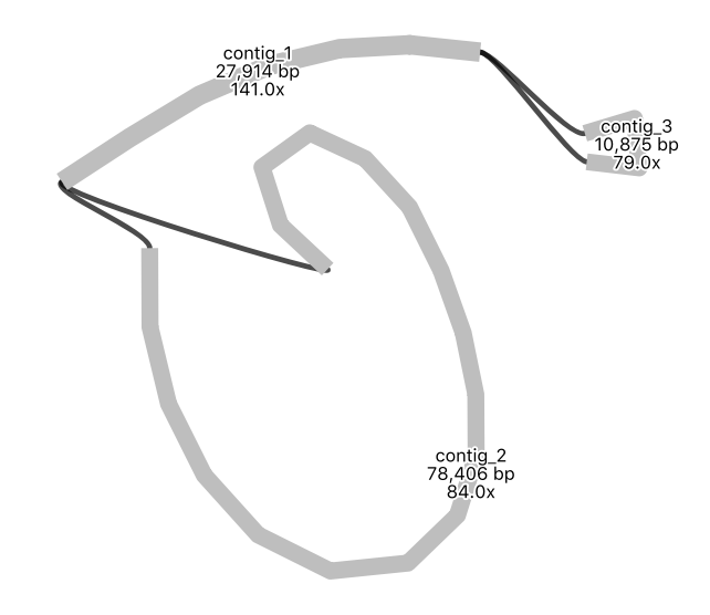Open image in new tab

Note: a newer version of the Flye assembly tool now resolves this assembly into a single circle.

Question

What is your interpretation of this assembly graph?

Solution

One interpretation is that this represents the typical circular chloroplast structure: There is a long single-copy region (the node of around 78,000 bp), connected to the inverted repeat (a node of around 28,000 bp), connected to the short single-copy region (of around 11,000 bp). In the graph, each end loop is a single-copy region (either long or short) and the centre bar is the collapsed inverted repeat which should have about twice the sequencing depth.

Comment: Further Learning

• Repeat the Flye assembly with different parameters, and/or a filtered read set.
• You can also try repeating the Flye assembly with an earlier version of the tool, to see the difference it makes. In the tool panel for Flye, click on the ‘Versions’ button at the top to change.
• Try an alternative assembly tool, such as Canu or Unicycler.

Polish assembly

Short illumina reads are more accurate the nanopore reads. We will use them to correct errors in the nanopore assembly.

First, we will map the short reads to the assembly and create an alignment file.

Hands-on: Map reads

1. Map with BWA-MEM ( Galaxy version 0.7.17.1):
   • “Will you select a reference genome from your history”: Use a genome from history
   • “Use the following dataset as the reference sequence”: flye-assembly.fasta
   • “Algorithm for constructing the BWT index”: Auto. Let BWA decide
   • “Single or Paired-end reads”: Single
   • “Select fastq dataset”: sweet-potato-illumina-reduced.fastq
   • “Set read groups information?”: Do not set
   • “Select analysis mode”: Simple Illumina mode
2. Re-name output file:
   • Re-name this file illumina.bam

Next, we will compare the short reads to the assembly, and create a polished (corrected) assembly file.

Hands-on: Polish

1. pilon ( Galaxy version 1.20.1):
   • “Source for reference genome used for BAM alignments”: Use a genome from history
   • “Select a reference genome”: flye-assembly.fasta
   • “Type automatically determined by pilon”: Yes
   • “Input BAM file”: illumina.bam
   • “Variant calling mode”: No
   • “Create changes file”: Yes
2. View output:
   • What is in the changes file?
   • Rename the fasta output to polished-assembly.fasta

   Tip: Renaming a dataset

   • Click on the galaxy-pencil pencil icon for the dataset to edit its attributes
   • In the central panel, change the Name field to polished-assembly.fasta
   • Click the Save button

3. Fasta Statistics ( Galaxy version 1.0.1)
   • Find and run the tool called “Fasta statistics” on both the original flye assembly and the polished version.

Question

How does the polished assembly compare to the unpolished assembly?

Solution

This will depend on the settings, but as an example: your polished assembly might be about 10-15 Kbp longer. Nanopore reads can have homopolymer deletions - a run of AAAA may be interpreted as AAA - so the more accurate illumina reads may correct these parts of the long-read assembly. In the changes file, there may be a lot of cases showing a supposed deletion (represented by a dot) being corrected to a base.

Optional further steps:

• Run a second round (or more) of Pilon polishing. Keep track of file naming; you will need to generate a new bam file first before each round of Pilon.
• Run an alternative polishing tool, such as Racon. This uses the long reads themselves to correct the long-read (Flye) assembly. It would be better to run this tool on the Flye assembly before running Pilon, rather than after Pilon.

Annotate the assembly

We can now annotate our assembled genome with information about genomic features.

• A chloroplast genome annotation tool is not yet available in Galaxy; for an approximation, here we can use the tool for bacterial genome annotation, Prokka.

Hands-on: Annotate with Prokka

1. Prokka ( Galaxy version 1.14.5+galaxy0) with the following parameters (leave everything else unchanged)
   • param-file “contigs to annotate”: polished-assembly.fasta
2. View output:
   • The GFF and GBK files contain all of the information about the features annotated (in different formats.)
   • The .txt file contains a summary of the number of features annotated.
   • The .faa file contains the protein sequences of the genes annotated.
   • The .ffn file contains the nucleotide sequences of the genes annotated.

Alternatively, you might want to use a web-based tool designed for chloroplast genomes.

• One option is the GeSeq tool, described here. Skip this step if you have already used Prokka above.

Hands-on: Annotate with GeSeq

• Download polished-assembly.fasta to your computer (click on the file in your history; then click on the disk icon).
• In a new browser tab, go to Chlorobox where we will use the GeSeq tool (Tillich et al. 2017) to annotate our sequence.
• Upload the fasta file there. Information about how to use the tool is available on the page.
• Once the annotation is completed, download the required files.
• In Galaxy, import the annotation GFF3 file.

Now make a JBrowse file to view the annotations (the GFF3 file - produced from either Prokka or GeSeq) under the assembly (the polished-assembly.fasta file).

Hands-on: View annotations

1. JBrowse genome browser ( Galaxy version 1.16.4+galaxy3):
   • “Reference genome to display”: Use a genome from history
     • “Select a reference genome”: polished-assembly.fasta
   • “Produce Standalone Instance”: Yes
   • “Genetic Code”: 11. The Bacterial, Archaeal and Plant Plastid Code
   • “JBrowse-in-Galaxy Action”: New JBrowse instance
   • “Insert Track Group”
     • “Insert Annotation Track”
       • “Track Type”: GFF/GFF3/BED Features
       • “GFF/GFF3/BED Track Data”: the GFF3 file
       • Leave the other track features as default
2. Re-name output file:
   • JBrowse may take a few minutes to run. There is one output file: re-name it view-annotations
3. View output:
   • Click on the eye icon to view the annotations file.
   • Select the right contig to view, in the drop down box.
   • Zoom out (with the minus button) until annotations are visible.

Here is an embedded snippet showing JBrowse and the annotations:

Open JBrowse in a new tab

View reads

We will look at the original sequencing reads mapped to the genome assembly. In this tutorial, we will import very cut-down read sets so that they are easier to view.

Hands-on: Import cut-down read sets

1. Import from Zenodo or a data library (ask your instructor):
   • FASTQ file with illumina reads: sweet-potato-chloroplast-illumina-tiny.fastq
   • FASTQ file with nanopore reads: sweet-potato-chloroplast-nanopore-tiny.fastq
   • Note: these are the “tiny” files, not the “reduced” files we imported earlier.

     https://zenodo.org/record/3567224/files/sweet-potato-chloroplast-illumina-tiny.fastq
     https://zenodo.org/record/3567224/files/sweet-potato-chloroplast-nanopore-tiny.fastq
     

Hands-on: Map the reads to the assembly

• Map the Illumina reads (the new “tiny” dataset) to the polished-assembly.fasta, the same way we did before, using bwa mem.
• This creates one output file: re-name it illumina-tiny.bam
• Map the Nanopore reads (the new “tiny” dataset) to the polished-assembly.fasta. The settings will be the same, except Select analysis mode should be Nanopore
• This creates one output file: re-name it nanopore-tiny.bam

Hands-on: Visualise mapped reads

1. JBrowse genome browser ( Galaxy version 1.16.4+galaxy3):
   • “Reference genome to display”: Use a genome from history
     • “Select a reference genome”: polished-assembly.fasta
   • “Produce Standalone Instance”: Yes
   • “Genetic Code”: 11. The Bacterial, Archaeal and Plant Plastid Code
   • “JBrowse-in-Galaxy Action”: New JBrowse instance
   • “Insert Track Group”
     • “Insert Annotation Track”
       • “Track Type”: BAM pileups
       • “BAM track data”: nanopore-tiny.bam
       • “Autogenerate SNP track”: No
       • Leave the other track features as default
     • “Insert Annotation Track”.
       • “Track Type”: BAM pileups
       • “BAM track data”: illumina-tiny.bam
       • “Autogenerate SNP track”: No
       • Leave the other track features as default
2. Re-name output file:
   • JBrowse may take a few minutes to run. There is one output file: re-name it assembly-and-reads
3. View output:
   • Click on the eye icon to view. (For more room, collapse Galaxy side menus with corner < > signs).
   • Make sure the bam files are ticked in the left hand panel.
   • Choose a contig in the drop down menu. Zoom in and out with + and - buttons.

Here is an embedded snippet showing JBrowse and the mapped reads:

Open JBrowse in a new tab

Question

1. What are the differences between the nanopore and the illumina reads?
2. What are some reasons that the read coverage may vary across the reference genome?

Solution

1. Nanopore reads are longer and have a higher error rate.
2. There may be lots of reasons for varying read coverage. Some possibilities: In areas of high read coverage: this region may be a collapsed repeat. In areas of low or no coverage: this region may be difficult to sequence; or, this region may be a misassembly.

• To learn more about JBrowse and its features, see the Genomic Data Visualisation with JBrowse tutorial

Repeat with new data

Optional extension exercise

We can assemble another chloroplast genome using sequence data from a different plant species: the snow gum, Eucalyptus pauciflora. This data is from Wang et al. 2018. It is a subset of the original FASTQ read files (Illumina - SRR7153063, Nanopore - SRR7153095).

Hands-on: Assembly and annotation

• Get data: at this Zenodo link, then upload to Galaxy.
• Check reads: Run Nanoplot on the nanopore reads.
• Assemble: Use Flye to assemble the nanopore reads, then get Fasta statistics Note: this may take several hours.
• Polish assembly: Use Pilon to polish the assembly with short Illumina reads. Note: Don’t forget to map these Illumina reads to the assembly first using bwa-mem, then use the resulting bam file as input to Pilon.
• Annotate: Use the GeSeq tool at Chlorobox or the Prokka tool within Galaxy.
• View annotations:Use JBrowse to view the assembled, annotated genome.

Conclusion

Key points

• A chloroplast genome can be assembled with long reads and polished with short reads

• The assembly graph is useful to look at and think about genomic structure

• We can map raw reads back to the assembly and investigate areas of high or low read coverage

• We can view an assembly, its mapped reads, and its annotations in JBrowse

Frequently Asked Questions

References

1. Tillich, M., P. Lehwark, T. Pellizzer, E. S. Ulbricht-Jones, A. Fischer et al., 2017 GeSeq – versatile and accurate annotation of organelle genomes. Nucleic Acids Research 45: W6–W11. 10.1093/nar/gkx391
2. Wang, W., M. Schalamun, A. Morales-Suarez, D. Kainer, B. Schwessinger et al., 2018 Assembly of chloroplast genomes with long- and short-read data: a comparison of approaches using Eucalyptus pauciflora as a test case. BMC Genomics 19: 10.1186/s12864-018-5348-8
3. Zhou, C., T. Duarte, R. Silvestre, G. Rossel, R. O. M. Mwanga et al., 2018 Insights into population structure of East African sweetpotato cultivars from hybrid assembly of chloroplast genomes. Gates Open Research 2: 41. 10.12688/gatesopenres.12856.1

Feedback

Did you use this material as an instructor? Feel free to give us feedback on how it went.
Did you use this material as a learner or student? Click the form below to leave feedback.

Citing this Tutorial

1. Anna Syme, Chloroplast genome assembly (Galaxy Training Materials). https://training.galaxyproject.org/training-material/topics/assembly/tutorials/chloroplast-assembly/tutorial.html Online; accessed TODAY
2. Hiltemann, Saskia, Rasche, Helena et al., 2023 Galaxy Training: A Powerful Framework for Teaching! PLOS Computational Biology 10.1371/journal.pcbi.1010752
3. Batut et al., 2018 Community-Driven Data Analysis Training for Biology Cell Systems 10.1016/j.cels.2018.05.012

BibTeX

@misc{assembly-chloroplast-assembly,
author = "Anna Syme",
	title = "Chloroplast genome assembly (Galaxy Training Materials)",
	year = "",
	month = "",
	day = ""
	url = "\url{https://training.galaxyproject.org/training-material/topics/assembly/tutorials/chloroplast-assembly/tutorial.html}",
	note = "[Online; accessed TODAY]"
}
@article{Hiltemann_2023,
	doi = {10.1371/journal.pcbi.1010752},
	url = {https://doi.org/10.1371%2Fjournal.pcbi.1010752},
	year = 2023,
	month = {jan},
	publisher = {Public Library of Science ({PLoS})},
	volume = {19},
	number = {1},
	pages = {e1010752},
	author = {Saskia Hiltemann and Helena Rasche and Simon Gladman and Hans-Rudolf Hotz and Delphine Larivi{\`{e}}re and Daniel Blankenberg and Pratik D. Jagtap and Thomas Wollmann and Anthony Bretaudeau and Nadia Gou{\'{e}} and Timothy J. Griffin and Coline Royaux and Yvan Le Bras and Subina Mehta and Anna Syme and Frederik Coppens and Bert Droesbeke and Nicola Soranzo and Wendi Bacon and Fotis Psomopoulos and Crist{\'{o}}bal Gallardo-Alba and John Davis and Melanie Christine Föll and Matthias Fahrner and Maria A. Doyle and Beatriz Serrano-Solano and Anne Claire Fouilloux and Peter van Heusden and Wolfgang Maier and Dave Clements and Florian Heyl and Björn Grüning and B{\'{e}}r{\'{e}}nice Batut and},
	editor = {Francis Ouellette},
	title = {Galaxy Training: A powerful framework for teaching!},
	journal = {PLoS Comput Biol} Computational Biology}
}

                   

Galaxy Administrators: Install the missing tools

You can use Ephemeris's shed-tools install command to install the tools used in this tutorial.

shed-tools install [-g GALAXY] [-a API_KEY] -t <(curl https://training.galaxyproject.org/training-material/api/topics/assembly/tutorials/chloroplast-assembly/tutorial.json | jq .admin_install_yaml -r)

Alternatively you can copy and paste the following YAML

---
install_tool_dependencies: true
install_repository_dependencies: true
install_resolver_dependencies: true
tools:
- name: flye
  owner: bgruening
  revisions: 3ee0ef312022
  tool_panel_section_label: Assembly
  tool_shed_url: https://toolshed.g2.bx.psu.edu/
- name: prokka
  owner: crs4
  revisions: bf68eb663bc3
  tool_panel_section_label: Annotation
  tool_shed_url: https://toolshed.g2.bx.psu.edu/
- name: prokka
  owner: crs4
  revisions: 111884f0d912
  tool_panel_section_label: Annotation
  tool_shed_url: https://toolshed.g2.bx.psu.edu/
- name: bwa
  owner: devteam
  revisions: 3fe632431b68
  tool_panel_section_label: Mapping
  tool_shed_url: https://toolshed.g2.bx.psu.edu/
- name: bandage
  owner: iuc
  revisions: b2860df42e16
  tool_panel_section_label: Graph/Display Data
  tool_shed_url: https://toolshed.g2.bx.psu.edu/
- name: bandage
  owner: iuc
  revisions: 94fe43e75ddc
  tool_panel_section_label: Graph/Display Data
  tool_shed_url: https://toolshed.g2.bx.psu.edu/
- name: fasta_stats
  owner: iuc
  revisions: 9c620a950d3a
  tool_panel_section_label: FASTA/FASTQ
  tool_shed_url: https://toolshed.g2.bx.psu.edu/
- name: fasta_stats
  owner: iuc
  revisions: 0dbb995c7d35
  tool_panel_section_label: FASTA/FASTQ
  tool_shed_url: https://toolshed.g2.bx.psu.edu/
- name: jbrowse
  owner: iuc
  revisions: 2bb2e07a7a21
  tool_panel_section_label: Graph/Display Data
  tool_shed_url: https://toolshed.g2.bx.psu.edu/
- name: jbrowse
  owner: iuc
  revisions: 17359b808b01
  tool_panel_section_label: Graph/Display Data
  tool_shed_url: https://toolshed.g2.bx.psu.edu/
- name: nanoplot
  owner: iuc
  revisions: edbb6c5028f5
  tool_panel_section_label: Nanopore
  tool_shed_url: https://toolshed.g2.bx.psu.edu/
- name: pilon
  owner: iuc
  revisions: 11e5408fd238
  tool_panel_section_label: Assembly
  tool_shed_url: https://toolshed.g2.bx.psu.edu/

Feedback

5 stars	17
4 stars	8
3 stars	1
2 stars	1

May 2023

• 5 stars: Liked: Interesting genome for tutorial and explanation of how to do long read assembly with short read polishing.

March 2022

• 5 stars: Disliked: pictures - screenshots can be added
• 4 stars: Liked: I learnt new tools that i haven't used before
• 5 stars: Liked: i liked on how to polish nano-pore reads
• 5 stars: Liked: Very easy to use and effective
• 5 stars: Liked: good intro course on assembly Disliked: some more theory about polishing and why
• 5 stars: Liked: All aspect Disliked: Not much improvement

December 2021

• 5 stars: Disliked: Circos plot of the data should also be included.

November 2021

• 5 stars: Liked: Very assertive and good guidance Disliked: More intuitive guidance

July 2021

• 5 stars: Liked: The overall training session was really nice. Disliked: However, some more information regarding the viewing in Jbrowse should be discussed like what to analyse in Jbrowse, how to spot irregularities and how to spot meaningful data? What kind of useful data can be visualized or can we get from the visualization in the Jbrowse.

June 2021

• 4 stars: Liked: The idea of comparing long and short reads and how to use short reads to polish the results Disliked: It would be great if there was a little explanation of how the tools work

February 2021

• 5 stars: Liked: I´d like to know how I can get a unique assemble using more than one pair of Illumina reads for the same DNA, for example the same bacterial strain. It is possible?
• 5 stars: Liked: Loved the self training with new data at the end. Helps user create a workflow to re run the steps rapidly and compare results. The tutorials were very clear and easy to understand
• 5 stars: Liked: Clear and easy

January 2021

• 2 stars: Liked: Clear Explanations Disliked: I noticed the "Note: this tool is heuristic; your results may differ slightly from the results here, and if repeated." But mine only showed one contig, with a length of 158kbp. I would consider this very different, not slightly different. Maybe add a few more examples of "slightly different" results I am running the tool again to see what I get. Additionally it took a long time to run this tool; almost an hour. So it would be nice to know approximately how long a tool is going to take, (given the fastq file & runtime parameters), or maybe show the log file while it is running (assuming the actual tool writes to the log file rather than just storing the info in memory and writing the log at the end...)