Generating a single cell matrix using Alevin and combining datasets (bash + R)
| Author(s) |
|
| Editor(s) |
|
| Tester(s) |
|
| Reviewers |
|
OverviewQuestions:
Objectives:
I have some single cell FASTQ files I want to analyse. Where do I start?
How to generate a single cell matrix using command line?
Requirements:
Generate a cellxgene matrix for droplet-based single cell sequencing data
Interpret quality control (QC) plots to make informed decisions on cell thresholds
Find relevant information in GTF files for the particulars of their study, and include this in data matrix metadata
Time estimation: 2 hoursSupporting Materials:Published: Dec 8, 2023Last modification: Apr 22, 2025License: Tutorial Content is licensed under Creative Commons Attribution 4.0 International License. The GTN Framework is licensed under MITpurl PURL: https://gxy.io/GTN:T00378rating Rating: 1.0 (0 recent ratings, 1 all time)version Revision: 5
Introduction
This tutorial is part of Single-cell RNA-seq: Case Study series and focuses on generating a single cell matrix using Alevin (Srivastava et al. 2019) in the bash command line. It is a replication of the previous tutorial and will guide you through the same steps that you followed in the previous tutorial and will give you more understanding of what is happening ‘behind the scenes’ or ‘inside the tools’ if you will. In this tutorial, we will go from raw FASTQ files to a cell x gene data matrix in SCE (SingleCellExperiment) format. We will perform the following steps:
- Getting the appropriate files
- Making a transcript-to-gene ID mapping
- Creating Salmon index
- Quantification of transcript expression using Alevin
- Creating Summarized Experiment from the Alevin output
- Adding metadata
- Combining samples data
Warning: This tutorial is for teaching purposesWe created this tutorial as a gateway to coding to demonstrate what happens behind the Galaxy buttons in the corresponding tutorial. This is why we are using massively subsampled data - it’s only for demonstration purposes. If you want to perform this tutorial fully on your own data, you will need another compute power because it’s simply not going to scale here. You can always use the Galaxy buttons’ Alevin version which has large memory and few cores dedicated.
Launching JupyterLab
Warning: Data uploads & JupyterLabThere are a few ways of importing and uploading data into JupyterLab. You might find yourself accidentally doing this differently than the tutorial, and that’s ok. There are a few key steps where you will call files from a location - if these don’t work for you, check that the file location is correct and change accordingly!
Hands On: Launch JupyterLabCurrently JupyterLab in Galaxy is available on Live.useGalaxy.eu, usegalaxy.org and usegalaxy.eu.
Hands On: Run JupyterLab
- Interactive Jupyter Notebook. Note that on some Galaxies this is called Interactive JupyTool and notebook:
- Click Run Tool
The tool will start running and will stay running permanently
This may take a moment, but once the
Executed notebookin your history is orange, you are up and running!- On the left menu bar you should see the Interactive Tools Icon now. Click on it to open the Active Interactive Tools and locate the JupyterLab instance you started.
- Click on your JupyterLab instance (JupyTool interactive tool)
If JupyterLab is not available on the Galaxy instance:
- Start Try JupyterLab
Comment: JupyterLab Notebook version on usegalaxy.euPlease note that there might be slight differences in the performance depending on the notebook version that you use. You can check the version by clicking on tool-versions Versions button. To date, the newest version is 1.0.1 - the conda installation is much quicker there, so we recommend using that version when following this tutorial.
Welcome to JupyterLab!
Warning: Danger: You can lose data!Do NOT delete or close this notebook dataset in your history. YOU WILL LOSE IT!
Open the notebook
You have two options for how to proceed with this JupyterLab tutorial - you can run the tutorial from a pre-populated notebook, or you can copy and paste the code for each step into a fresh notebook and run it. The initial instructions for both options are below.
Hands On: Option 1 (recommended): Open the notebook directly in JupyterLab
- Open a
Terminalin JupyterLab with File -> New -> Terminal (you will use terminal in a moment again to install required packages!)
- Run
wget https://training.galaxyproject.org/training-material/topics/single-cell/tutorials/alevin-commandline/single-cell-alevin-commandline.ipynb- Select the notebook that appears in the list of files on the left.
Remember that you can also download this notebook Jupyter Notebook from the galaxy_instance Supporting Materials in the Overview box at the beginning of this tutorial.

Hands On: Option 2: Creating a notebook
If you are in the Launcher window, Select the Bash icon under Notebook (to open a new Launcher go to File -> New Launcher).
Save your file (File: Save, or click the galaxy-save Save icon at the top left)
If you right click on the file in the folder window at the left, you can rename your file
whateveryoulike.ipynb
Warning: You should Save frequently!This is both for good practice and to protect you in case you accidentally close the browser. Your environment will still run, so it will contain the last saved notebook you have. You might eventually stop your environment after this tutorial, but ONLY once you have saved and exported your notebook (more on that at the end!) Note that you can have multiple notebooks going at the same time within this JupyterLab, so if you do, you will need to save and export each individual notebook. You can also download them at any time.
Let’s crack on!
Warning: Notebook-based tutorials can give different outputsThe nature of coding pulls the most recent tools to perform tasks. This can - and often does - change the outputs of an analysis. Be prepared, as you are unlikely to get outputs identical to a tutorial if you are running it in a programming environment like a Jupyter Notebook or R-Studio. That’s ok! The outputs should still be pretty close.
Setting up the environment
Alevin is a tool integrated with the Salmon software, so first we need to get Salmon. You can install Salmon using conda, but in this tutorial we will show an alternative method - downloading the pre-compiled binaries from the releases page. Note that binaries are usually compiled for specific CPU architectures, such as the 64-bit (x86_64) machine release referenced below .
wget -nv https://github.com/COMBINE-lab/salmon/releases/download/v1.10.0/salmon-1.10.0_linux_x86_64.tar.gz
Once you’ve downloaded a specific binary (here we’re using version 1.10.0), just extract it like so:
tar -xvzf salmon-1.10.0_linux_x86_64.tar.gz
As mentioned, installing salmon using conda is also an option, and you can do it using the following command in the terminal:
conda install -c conda-forge -c bioconda salmonHowever, for this tutorial, it would be easier and quicker to use the downloaded pre-compiled binaries, as shown above.
We’re going to use Alevin for demonstration purposes, but we do not endorse one method over another.
Get Data
We continue working on the same example data - a very small subset of the reads in a mouse dataset of fetal growth restriction Bacon et al. 2018 (see the study in Single Cell Expression Atlas and the project submission). For the purposes of this tutorial, the datasets have been subsampled to only 50k reads (around 1% of the original files). Those are two fastq files - one with transcripts and the another one with cell barcodes. You can download the files by running the code below:
wget -nv https://zenodo.org/records/10116786/files/transcript_701.fastq
wget -nv https://zenodo.org/records/10116786/files/barcodes_701.fastq
QuestionHow to differentiate between the two files if they are just called ‘Read 1’ and ‘Read 2’?
The file which contains the cell barcodes and UMI is significantly shorter (indeed, 20 bp!) compared to the other file containing longer, transcript read. For ease, we will use explicit file names.
Additionally, to map your reads, you will need a transcriptome to align against (a FASTA) as well as the gene information for each transcript (a gtf) file. These files are included in the data import step below. You can also download these for your species of interest from Ensembl.
wget -c https://zenodo.org/record/4574153/files/Mus_musculus.GRCm38.100.gtf.gff -O GRCm38_gtf.gff
wget -c https://zenodo.org/record/4574153/files/Mus_musculus.GRCm38.cdna.all.fa.fasta -O GRCm38_cdna.fasta
Why do we need FASTA and GTF files? To generate gene-level quantifications based on transcriptome quantification, Alevin and similar tools require a conversion between transcript and gene identifiers. We can derive a transcript-gene conversion from the gene annotations available in genome resources such as Ensembl. The transcripts in such a list need to match the ones we will use later to build a binary transcriptome index. If you were using spike-ins, you’d need to add these to the transcriptome and the transcript-gene mapping.
We will use the murine reference annotation as retrieved from Ensembl (GRCm38 or mm10) in GTF format. This annotation contains gene, exon, transcript and all sorts of other information on the sequences. We will use these to generate the transcript-gene mapping by passing that information to a tool that extracts just the transcript identifiers we need.
Finally, we will download some files for later so that you don’t have to switch kernels again - that’s an Alevin output folder for another sample!
wget https://zenodo.org/records/10116786/files/alevin_output_702.zip
unzip alevin_output_702.zip
Generate a transcript to gene map and filtered FASTA
We will now install the package atlas-gene-annotation-manipulation to help us generate the files required for Salmon and Alevin.
conda install -y -c conda-forge -c bioconda atlas-gene-annotation-manipulation
After the installation is completed, you can execute the code cell below and while it’s running, I’ll explain all the parameters we set here.
gtf2featureAnnotation.R -g GRCm38_gtf.gff -c GRCm38_cdna.fasta -d "transcript_id" -t "transcript" -f "transcript_id" -o map -l "transcript_id,gene_id" -r -e filtered_fasta
In essence, gtf2featureAnnotation.R script takes a GTF annotation file and creates a table of annotation by feature, optionally filtering a cDNA file supplied at the same time. Therefore the first parameter -g stands for “gtf-file” and requires a path to a valid GTF file. Then -c takes a cDNA file for extracting meta info and/or filtering - that’s our FASTA! Where –parse-cdnas (that’s our -c) is specified, we need to specify, using -d, which field should be used to compare to identfiers from the FASTA. We set that to “transcript_id” - feel free to inspect the GTF file to explore other attributes. We pass the same value in -f, meaning first-field, ie. the name of the field to place first in output table. To specify which other fields to retain in the output table, we provide comma-separated list of those fields, and since we’re only interested in transcript to gene map, we put those two names (“transcript_id,gene_id”) into -l. -t stands for the feature type to use, and in our case we’re using “transcript”. Guess what -o is! Indeed, that’s the output annotation table - here we specify the file path of our transcript to gene map. We will also have another output denoted by -e and that’s the path to a filtered FASTA. Finally, we also put -r which is there only to suppress header on output. Summarising, output will be a an annotation table, and a FASTA-format cDNAs file with unannotated transcripts removed.
Why filtered FASTA? Sometimes it’s important that there are no transcripts in a FASTA-format transcriptome that cannot be matched to a transcript/gene mapping. Salmon, for example, used to produce errors when this mismatch was present. We can synchronise the cDNA file by removing mismatches as we have done above.
Generate a transcriptome index
We will use Salmon in mapping-based mode, so first we have to build a Salmon index for our transcriptome. We will run the Salmon indexer as so:
salmon-latest_linux_x86_64/bin/salmon index -t filtered_fasta -i salmon_index -k 31
Where -t stands for our filtered FASTA file, and -i is the output of the mapping-based index. To build it, the function is using an auxiliary k-mer hash over k-mers of length 31. While the mapping algorithms will make use of arbitrarily long matches between the query and reference, the k size selected here will act as the minimum acceptable length for a valid match. Thus, a smaller value of k may slightly improve sensitivity. We find that a k of 31 seems to work well for reads of 75bp or longer, but you might consider a smaller k if you plan to deal with shorter reads. Also, a shorter value of k may improve sensitivity even more when using selective alignment (enabled via the –validateMappings flag). So, if you are seeing a smaller mapping rate than you might expect, consider building the index with a slightly smaller k.
To be able to search a transcriptome quickly, Salmon needs to convert the text (FASTA) format sequences into something it can search quickly, called an ‘index’. The index is in a binary rather than human-readable format, but allows fast lookup by Alevin. Because the types of biological and technical sequences we need to include in the index can vary between experiments, and because we often want to use the most up-to-date reference sequences from Ensembl or NCBI, we can end up re-making the indices quite often.
Use Alevin
Time to use Alevin now! Alevin works under the same indexing scheme (as Salmon) for the reference, and consumes the set of FASTA/Q files(s) containing the Cellular Barcode(CB) + Unique Molecule identifier (UMI) in one read file and the read sequence in the other. Given just the transcriptome and the raw read files, Alevin generates a cell-by-gene count matrix (in a fraction of the time compared to other tools).
Alevin works in two phases. In the first phase it quickly parses the read file containing the CB and UMI information to generate the frequency distribution of all the observed CBs, and creates a lightweight data-structure for fast-look up and correction of the CB. In the second round, Alevin utilizes the read-sequences contained in the files to map the reads to the transcriptome, identify potential PCR/sequencing errors in the UMIs, and performs hybrid de-duplication while accounting for UMI collisions. Finally, a post-abundance estimation CB whitelisting procedure is done and a cell-by-gene count matrix is generated.
Alevin can be run using the following command:
salmon-latest_linux_x86_64/bin/salmon alevin -l ISR -1 barcodes_701.fastq -2 transcript_701.fastq --dropseq -i salmon_index -p 10 -o alevin_output --tgMap map --freqThreshold 3 --keepCBFraction 1 --dumpFeatures
All the required input parameters are described in the documentation, but for the ease of use, they are presented below as well:
-l: library type (same as Salmon), we recommend using ISR for both Drop-seq and 10x-v2 chemistry.
-1: CB+UMI file(s), alevin requires the path to the FASTQ file containing CB+UMI raw sequences to be given under this command line flag. Alevin also supports parsing of data from multiple files as long as the order is the same as in -2 flag. That’s our barcodes_701.fastq file.
-2: Read-sequence file(s), alevin requires the path to the FASTQ file containing raw read-sequences to be given under this command line flag. Alevin also supports parsing of data from multiple files as long as the order is the same as in -1 flag. That’s our transcript_701.fastq file.
--dropseq/--chromium/--chromiumV3: the protocol, this flag tells the type of single-cell protocol of the input sequencing-library. This is a study using the Drop-seq chemistry, so we specify that in the flag.
-i: index, file containing the salmon index of the reference transcriptome, as generated by salmon index command.
-p: number of threads, the number of threads which can be used by alevin to perform the quantification, by default alevin utilizes all the available threads in the system, although we recommend using ~10 threads which in our testing gave the best memory-time trade-off.
-o: output, path to folder where the output gene-count matrix (along with other meta-data) would be dumped. We simply call it alevin_output
--tgMap: transcript to gene map file, a tsv (tab-separated) file — with no header, containing two columns mapping of each transcript present in the reference to the corresponding gene (the first column is a transcript and the second is the corresponding gene). In our case, that’s map_code generated by using gtf2featureAnnotation.R function.
--freqThreshold- minimum frequency for a barcode to be considered. We’ve chosen 3 as this will only remove cell barcodes with a frequency of less than 3, a low bar to pass but useful way of avoiding processing a bunch of almost certainly empty barcodes.
--keepCBFraction- fraction of cellular barcodes to keep. We’re using 1 to quantify all!
--dumpFeatures- if activated, alevin dumps all the features used by the CB classification and their counts at each cell level. It’s generally used in pair with other command line flags.
We have also added some additional parameters (--freqThreshold, --keepCBFraction) and their values are derived from the Alevin Galaxy tutorial after QC to stop Alevin from applying its own thresholds. However, if you’re not sure what value to pick, you can simply allow Alevin to make its own calls on what constitutes empty droplets.
This tool will take a while to run. Alevin produces many file outputs, not all of which we’ll use. You can refer to the Alevin documentation if you’re curious what they all are, you can look through all the different files to find information such as the mapping rate, but we’ll just pass the whole output folder directory for downstream analysis.
Question
- Can you find the information what was the mapping rate?
- How many transcripts did Alevin find?
- As mentioned above, in alevin_output folder there will be many different files, including the log files. To check the mapping rate, go to alevin_output -> logs and open salmon_quant file. There you will find not only information about mapping rate, but also many more, calculated at salmon indexing step.
- Alevin log can be found in alevin_output -> alevin and the file name is also alevin. You can find many details about the alevin process there, including the number of transcripts found.
Warning: Process stoppingThe command above will display the log of the process and will say “Analyzed X cells (Y% of all)”. For some reason, running Alevin may sometimes cause problems in Jupyter Notebook and this process will stop and not go to completion. This is the reason why we use hugely subsampled dataset here - bigger ones couldn’t be fully analysed (they worked fine locally though). The dataset used in this tutorial shouldn’t make any issues when you’re using Jupyter notebook through galaxy.eu, however might not work properly on galaxy.org. If you’re accessing Jupyter notebook via galaxy.eu and alevin process stopped, just restart the kernel (in the upper left corner: Kernel -> Restart kernel…) and that should help. However, if it doesn’t, here are the alternatives:
- We prepared a Jupyter notebook with the same workflow as shown here, compatible with Google Collab. So if you have troubles with running the above step, you can use the notebook provided, upload it to your Google Collab and run the code there, following the tutorial on GTN.
- You can download the output folder that you would get as a result of running the code above. Simply run the code below.
# get the output folder from Alevin in case yours crashes
wget https://zenodo.org/records/13732502/files/alevin_output.zip
unzip alevin_output.zip
Alevin output to SummarizedExperiment
Let’s change gear a little bit. We’ve done the work in bash, and now we’re switching to R to complete the processing. To do so, you have to change Kernel to R (either click on Kernel -> Change Kernel... in the upper left corner of your JupyterLab or click on the displayed current kernel in the upper right corner and change it).
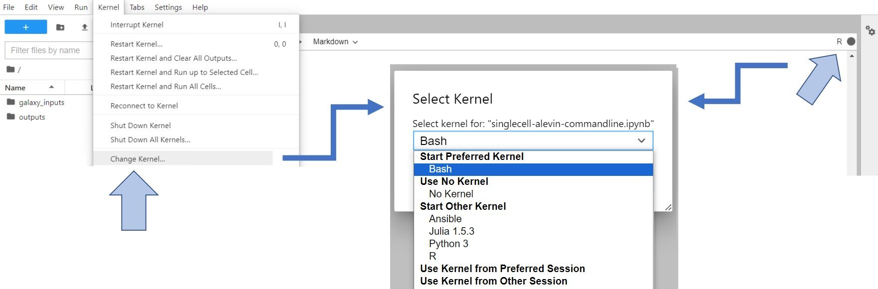 Open image in new tab
Now, when we are in the R environment, let’s install the packages required for this part - tximeta and DropletUtils:
system("conda install -y bioconductor-tximeta bioconductor-dropletutils", intern=TRUE)
Double check that the installation went fine:
require("tximeta")
require("DropletUtils")
If you encounter this error message while loading the library, you can try to install them with BiocManager, as shown below. Just replace “package_name” with either
tximetaorDropletUtils. Beware, it can take up to 25 minutes to run!# run the code below only if you cannot load tximeta library (or using notebook version 1.0.1) if (!require("BiocManager", quietly = TRUE)) install.packages("BiocManager") BiocManager::install("package_name") library("package_name")
The tximeta package created by Love et al. 2020 is used for import of transcript-level quantification data into R/Bioconductor and requires that the entire output of alevin is present and unmodified.
In the alevin_output -> alevin folder you can find the following files:
- quants_mat.gz- Compressed count matrix
- quants_mat_rows.txt- Row Index (CB-ids) of the matrix.
- quants_mat_cols.txt - Column Header (Gene-ids) of the matrix.
- quants_tier_mat.gz – Tier categorization of the matrix.
We will only focus on quants_mat.gz though. First, let’s specify the path to that file:
path <- 'alevin_output/alevin/quants_mat.gz'
We will specify the following arguments when running tximeta:
- ‘coldata’ a data.frame with at least two columns:
- files - character, paths of quantification files
- names - character, sample names
- ‘type’ - what quantifier was used (can be ‘salomon’, ‘alevin’, etc.)
With that we can create a dataframe and pass it to tximeta to create SummarizedExperiment object.
coldata <- data.frame(files = path, names="sample701")
alevin_se <- tximeta(coldata, type = "alevin")
Inspect the created object:
alevin_se
As you can see, rowData names and colData names are still empty. Before we add some metadata, we will first identify barcodes that correspond to non-empty droplets.
Identify barcodes that correspond to non-empty droplets
Some sub-populations of small cells may not be distinguished from empty droplets based purely on counts by barcode. Some libraries produce multiple ‘knees’ (see the Alevin Galaxy tutorial for multiple sub-populations. The emptyDrops method (Lun et al. 2019) has become a popular way of dealing with this. emptyDrops still retains barcodes with very high counts, but also adds in barcodes that can be statistically distinguished from the ambient profiles, even if total counts are similar.
EmptyDrops takes multiple arguments that you can read about in the documentation. However, in this case, we will only specify the following arguments:
m- A numeric matrix-like object - usually a dgTMatrix or dgCMatrix - containing droplet data prior to any filtering or cell calling. Columns represent barcoded droplets, rows represent genes.lower- A numeric scalar specifying the lower bound on the total UMI count, at or below which all barcodes are assumed to correspond to empty droplets.niters- An integer scalar specifying the number of iterations to use for the Monte Carlo p-value calculations.retain- A numeric scalar specifying the threshold for the total UMI count above which all barcodes are assumed to contain cells.
Let’s then extract the matrix from our alevin_se object. It’s stored in assays -> counts.
matrix_alevin <- assays(alevin_se)$counts
And now run emptyDrops:
# Identify likely cell-containing droplets
out <- emptyDrops(matrix_alevin, lower = 100, niters = 1000, retain = 20)
out
We also correct for multiple testing by controlling the false discovery rate (FDR) using the Benjamini-Hochberg (BH) method (Benjamini and Hochberg 1995). Putative cells are defined as those barcodes that have significantly poor fits to the ambient model at a specified FDR threshold. Here, we will use an FDR threshold of 0.01. This means that the expected proportion of empty droplets in the set of retained barcodes is no greater than 1%, which we consider to be acceptably low for downstream analyses.
is.cell <- out$FDR <= 0.01
sum(is.cell, na.rm=TRUE)                              # check how many cells left after filtering
We got rid of the background droplets containing no cells, so now we will filter the matrix that we passed on to emptyDrops, so that it corresponds to the remaining cells.
emptied_matrix <- matrix_alevin[,which(is.cell),drop=FALSE] # filter the matrix
From here, we can move on to adding metadata and we’ll return to emptied_matrix soon.
Adding cell metadata
The cells barcodes are stored in colnames. Let’s exctract them into a separate object:
barcode <- colnames(alevin_se)
Now, we can simply add those barcodes into colData names where we will keep the cell metadata. To do this, we will create a column called barcode in colData and pass the stored values into there.
colData(alevin_se)$barcode <- barcode
colData(alevin_se)
That’s only cell barcodes for now! However, after running emptyDrops, we generated lots of cell information that is currently stored in out object (Total, LogProb, PValue, Limited, FDR). Let’s add those values to cell metadata! Since we already have barcodes in there, we will simply bind the emptyDrops output to the existing dataframe:
colData(alevin_se) <- cbind(colData(alevin_se),out)
colData(alevin_se)
As you can see, the new columns were appended successfully and now the dataframe has 6 columns.
If you have a look at the Experimental Design from that study, you might notice that there is actually more information about the cells. The most important for us would be batch, genotype and sex, summarised in the small table below.
| Index | Batch | Genotype | Sex |
|---|---|---|---|
| N701 | 0 | wildtype | male |
| N702 | 1 | knockout | male |
| N703 | 2 | knockout | female |
| N704 | 3 | wildtype | male |
| N705 | 4 | wildtype | male |
| N706 | 5 | wildtype | male |
| N707 | 6 | knockout | male |
We are currently analysing sample N701, so let’s add its information from the table.
Batch
We will label batch as an integer - “0” for sample N701, “1” for N702 etc. The way to do it is creating a list with zeros of the length corresponding to the number of cells that we have in our SummarizedExperiment object, like so:
batch <- rep("0", length(colnames(alevin_se)))
And now create a batch slot in the colData names and append the batch list in the same way as we did with barcodes:
colData(alevin_se)$batch <- batch
colData(alevin_se)
A new column appeared, full of zeros - as expected!
Genotype
It’s all the same for genotype, but instead creating a list with zeros, we’ll create a list with string “wildtype” and append it into genotype slot:
genotype <- rep("wildtype", length(colnames(alevin_se)))
colData(alevin_se)$genotype <- genotype
Sex
You already know what to do, right? A list with string “male” and then adding it into a new slot!
sex <- rep("male", length(colnames(alevin_se)))
colData(alevin_se)$sex <- sex
Check if all looks fine:
colData(alevin_se)
3 new columns appeared with the information that we’ve just added - perfect! You can add any information you need in this way, as long as it’s the same for all the cells from one sample.
Adding gene metadata
The genes IDs are stored in rownames. Let’s exctract them into a separate object:
gene_ID <- rownames(alevin_se)
Analogically, we will add those genes IDs into rowData names which stores gene metadata. To do this, we will create a column called gene_ID in rowData and pass the stored values into there.
rowData(alevin_se)$gene_ID <- gene_ID
Adding genes symbols based on their IDs
Since gene symbols are much more informative than only gene IDs, we will add them to our metadata. We will base this annotation on Ensembl - the genome database – with the use of the library BioMart. We will use the archive Genome assembly GRCm38 to get the gene names. Please note that the updated version (GRCm39) is available, but some of the gene IDs are not in that EnsEMBL database. The code below is written in a way that it will work for the updated dataset too, but will produce ‘NA’ where the corresponding gene name couldn’t be found.
# get relevant gene names
library("biomaRt")                                      # load the BioMart library
ensembl.ids <- gene_ID
mart <- useEnsembl(biomart = "ENSEMBL_MART_ENSEMBL")    # connect to a specified BioMart database and dataset hosted by Ensembl
ensembl_m = useMart("ensembl", dataset="mmusculus_gene_ensembl")

# The line above connects to a specified BioMart database and dataset within this database.
# In our case we choose the mus musculus database and to get the desired Genome assembly GRCm38,
# we specify the host with this archive. If you want to use the most recent version of the dataset, just run:
# ensembl_m = useMart("ensembl", dataset="mmusculus_gene_ensembl")
Warning: Ensembl connection problemsSometimes you may encounter some connection issues with Ensembl. To improve performance Ensembl provides several mirrors of their site distributed around the globe. When you use the default settings for useEnsembl() your queries will be directed to your closest mirror geographically. In theory this should give you the best performance, however this is not always the case in practice. For example, if the nearest mirror is experiencing many queries from other users it may perform poorly for you. In such cases, the other mirrors should be chosen automatically.
genes <- getBM(attributes=c('ensembl_gene_id','external_gene_name'),
               filters = 'ensembl_gene_id',
               values = ensembl.ids,
               mart = ensembl_m)

# The line above retrieves the specified attributes from the connected BioMart database;
# 'ensembl_gene_id' are genes IDs,
# 'external_gene_name' are the genes symbols that we want to get for our values stored in ‘ensembl.ids’.
# see the resulting data
head(genes)
# replace IDs for gene names
gene_names <- ensembl.ids
count = 1
for (geneID in gene_names)
{
 index <- which(genes==geneID)    # finds an index of geneID in the genes object created by getBM()
 if (length(index)==0)            # condition in case if there is no corresponding gene name in the chosen dataset
  {
    gene_names[count] <- 'NA'
  }
  else
  {
    gene_names[count] <- genes$external_gene_name[index] 	# replaces gene ID by the corresponding gene name based on the found geneID’s index
  }
 count = count + 1                # increased count so that every element in gene_names is replaced
}
# add the gene names into rowData in a new column gene_name
rowData(alevin_se)$gene_name <- gene_names
# see the changes
rowData(alevin_se)
If you are working on your own data and it’s not mouse data, you can check available datasets for other species and just use relevant dataset in useMart() function.
listDatasets(mart) # available datasets
Flag mitochondrial genes
We can also flag mitochondrial genes. Usually those are the genes whose name starts with ‘mt-‘ or ‘MT-‘. Therefore, we will store those characters in mito_genes_names and then use grepl() to find those genes stored in gene_name slot.
mito_genes_names <- '^mt-|^MT-'                                    # how mitochondrial gene names can start
mito <- grepl(mito_genes_names, rowData(alevin_se)$gene_name)      # find mito genes
mito                                                               # see the resulting boolean list
Now we can add another slot in rowData and call it mito that will keep boolean values (true/false) to indicate which genes are mitochondrial.
rowData(alevin_se)$mito <- mito
rowData(alevin_se)
Subsetting the object
Let’s go back to the emptied_matrix object. Do you remember how many cells were left after filtering? We can check that by looking at the matrix’ dimensions:
dim(matrix_alevin)                                                  # check the dimension of the unfiltered matrix
dim(emptied_matrix)                                                 # check the dimension of the filtered matrix
We’ve gone from 3608 to 35 cells. We’ve filtered the matrix, but not our SummarizedExperiment. We can subset alevin_se based on the cells that were left after filtering. We will store them in a separate list, as we did with the barcodes:
retained_cells <- colnames(emptied_matrix)
retained_cells
And now we can subset our SummarizedExperiment based on the barcodes that are in the retained_cells list:
alevin_subset <- alevin_se[, colData(alevin_se)$barcode %in% retained_cells]
alevin_701 <- alevin_subset
alevin_701
And that’s our subset, ready for downstream analysis!
More datasets
We’ve done the analysis for one sample. But there are 7 samples in this experiment and it would be very handy to have all the information in one place. Therefore, you would need to repeat all the steps for the subsequent samples (that’s when you’ll appreciate wrapped tools and automation in Galaxy workflows!). To make your life easier, we will show you how to combine the datasets on smaller scale. Also, to save you some time, we’ve already run Alevin on sample 702 (also subsampled to 50k reads). Let’s quickly repeat the steps we performed in R to complete the analysis of sample 702 in the same way as we did with 701.
But first, we have to save the results of our hard work on sample 701!
Saving sample 701 data
Saving files is quite straightforward. Just specify which object you want to save and how you want the file to be named. Don’t forget the extension!
save(alevin_701, file = "alevin_701.rdata")
You will see the new file in the panel on the left.
Analysis of sample 702
Normally, at this point you would switch kernel to bash to run alevin, and then back to R to complete the analysis of another sample. Here, we are providing you with the alevin output for the next sample, which you have already downloaded and unzipped at the beginning of the tutorial when we were using bash.
Warning: Switching kernels & losing variablesBe aware that every time when you switch kernel, you will lose variables you store in the objects that you’ve created, unless you save them. Therefore, if you want to switch from R to bash, make sure you save your R objects! You can then load them anytime.
Above we described all the steps done in R and explained what each bit of code does. Below all those steps are in one block of code, so read carefully and make sure you understand everything!
## load libraries again ##
library(tximeta)
library(DropletUtils)
library(biomaRt)

## running tximeta ##
path2 <- 'alevin_output_702/alevin/quants_mat.gz'                                                    # path to alevin output for N702
alevin2 <- tximeta(coldata = data.frame(files = path2, names = "sample702"), type = "alevin")        # create SummarizedExperiment from Alevin output

## running emptyDrops ##
matrix_alevin2 <- assays(alevin2)$counts                                                             # extract matrix from SummarizedExperiment
out2 <- emptyDrops(matrix_alevin2, lower = 100, niters = 1000, retain = 20)                          # apply emptyDrops
is.cell2 <- out2$FDR <= 0.01                                                                         # apply FDR threshold
emptied_matrix2 <- matrix_alevin2[,which(is.cell2),drop=FALSE]                                       # subset the matrix to the cell-containing droplets

## adding cell metadata ##
barcode2 <- colnames(alevin2)
colData(alevin2)$barcode <- barcode2                                             # add barcodes

colData(alevin2) <- cbind(colData(alevin2),out2)                                 # add emptyDrops info

batch2 <- rep("1", length(colnames(alevin2)))
colData(alevin2)$batch <- batch2                                                # add batch info

genotype2 <- rep("wildtype", length(colnames(alevin2)))
colData(alevin2)$genotype <- genotype2                                          # add genotype info

sex2 <- rep("male", length(colnames(alevin2)))
colData(alevin2)$sex <- sex2                                                    # add sex info

## adding gene metadata ##
gene_ID2 <- rownames(alevin2)
rowData(alevin2)$gene_ID <- gene_ID2

# get relevant gene names
ensembl.ids2 <- gene_ID2
mart <- useEnsembl(biomart = "ENSEMBL_MART_ENSEMBL")    # connect to a specified BioMart database and dataset hosted by Ensembl
ensembl_m2 = useMart("ensembl", dataset="mmusculus_gene_ensembl")

genes2 <- getBM(attributes=c('ensembl_gene_id','external_gene_name'),
               filters = 'ensembl_gene_id',
               values = ensembl.ids2,
               mart = ensembl_m2)

# replace IDs for gene names
gene_names2 <- ensembl.ids2
count = 1
for (geneID in gene_names2)
{
 index <- which(genes2==geneID)    # finds an index of geneID in the genes object created by getBM()
 if (length(index)==0)            # condition in case if there is no corresponding gene name in the chosen dataset
  {
    gene_names2[count] <- 'NA'
  }
  else
  {
    gene_names2[count] <- genes2$external_gene_name[index] 	# replaces gene ID by the corresponding gene name based on the found geneID’s index
  }
 count = count + 1                # increased count so that every element in gene_names is replaced
}

rowData(alevin2)$gene_name <- gene_names2                              # add gene names to gene metadata

mito_genes_names <- '^mt-|^MT-'                                        # how mitochondrial gene names can start
mito2 <- grepl(mito_genes_names, rowData(alevin2)$gene_name)           # find mito genes
rowData(alevin2)$mito <- mito2                                         # add mitochondrial information to gene metadata

## create a subset of filtered object ##
retained_cells2 <- colnames(emptied_matrix2)
alevin_subset2 <- alevin2[, colData(alevin2)$barcode %in% retained_cells2]

alevin_702 <- alevin_subset2
alevin_702
Alright, another sample pre-processed!
Combining datasets
Pre-processed sample 702 is there, but keep in mind that if you switched kernels in the meantime, you still need to load sample 701 that was saved before switching kernels. It’s equally easy as saving the object:
load("alevin_701.rdata")
Check if it was loaded ok:
alevin_701
Now we can combine those two objects into one using one simple command:
alevin_combined <- cbind(alevin_701, alevin_702)
alevin_combined
If you have more samples, just append them in the same way. We won’t process another sample here, but pretending that we have third sample, we would combine it like this:
alevin_subset3 <- alevin_702                        # copy dataset for demonstration purposes
alevin_combined_demo <- cbind(alevin_combined, alevin_subset3)
alevin_combined_demo
You get the point, right? It’s important though that the rowData names and colData names are the same in each sample.
Saving and exporting the files
It is generally more common to use SingleCellExperiment format rather than SummarizedExperiment. The conversion is quick and easy, and goes like this:
library(SingleCellExperiment)                                 # might need to load this library
alevin_sce <- as(alevin_combined, "SingleCellExperiment")
alevin_sce
As you can see, all the embeddings have been successfully transfered during this conversion and believe me, SCE object will be more useful for you!
You’ve already learned how to save and load objects in Jupyter notebook, let’s then save the SCE file:
save(alevin_sce, file = "alevin_sce.rdata")
The last thing that might be useful is exporting the files into your Galaxy history. To do it… guess what! Yes - switching kernels again! But this time we choose Python 3 kernel and run the following command:
# that's Python now!
put("alevin_sce.rdata")
A new dataset should appear in your Galaxy history now.
Conclusion
Well done! In this tutorial we have:
- examined raw read data, annotations and necessary input files for quantification
- created an index in Salmon and run Alevin
- identified barcodes that correspond to non-empty droplets
- added gene and cell metadata
- applied the necessary conversion to pass these data to downstream processes.
As you might now appreciate, some tasks are much quicker and easier when run in the code, but the reproducibility and automation of Galaxy workflows is a huge advantage that helps in dealing with many samples more quickly and efficiently.
You've Finished the Tutorial
Key points
Create a SCE object from FASTQ files, including relevant gene and cell metadata, and do it all in Jupyter Notebook!
Frequently Asked Questions
Have questions about this tutorial? Have a look at the available FAQ pages and support channelsUseful literature
Further information, including links to documentation and original publications, regarding the tools, analysis techniques and the interpretation of results described in this tutorial can be found here.
References
- Benjamini, Y., and Y. Hochberg, 1995 Controlling the False Discovery Rate: A Practical and Powerful Approach to Multiple Testing. Journal of the Royal Statistical Society: Series B (Methodological) 57: 289–300. 10.1111/j.2517-6161.1995.tb02031.x
- Bacon, W. A., R. S. Hamilton, Z. Yu, J. Kieckbusch, D. Hawkes et al., 2018 Single-Cell Analysis Identifies Thymic Maturation Delay in Growth-Restricted Neonatal Mice. Frontiers in Immunology 9: 10.3389/fimmu.2018.02523
- Lun, A. T. L., and Samantha Riesenfeld, T. Andrews, T. P. Dao, T. Gomes et al., 2019 EmptyDrops: distinguishing cells from empty droplets in droplet-based single-cell RNA sequencing data. Genome Biology 20: 10.1186/s13059-019-1662-y
- Srivastava, A., L. Malik, T. Smith, I. Sudbery, and R. Patro, 2019 Alevin efficiently estimates accurate gene abundances from dscRNA-seq data. Genome Biology 20: 10.1186/s13059-019-1670-y
- Love, M. I., C. Soneson, P. F. Hickey, L. K. Johnson, N. T. Pierce et al., 2020 Tximeta: Reference sequence checksums for provenance identification in RNA-seq (M. Pertea, Ed.). PLOS Computational Biology 16: e1007664. 10.1371/journal.pcbi.1007664
Feedback
Did you use this material as an instructor? Feel free to give us feedback on how it went.
Did you use this material as a learner or student? Click the form below to leave feedback.

Citing this Tutorial
- Julia Jakiela, Wendi Bacon, Generating a single cell matrix using Alevin and combining datasets (bash + R) (Galaxy Training Materials). https://training.galaxyproject.org/training-material/topics/single-cell/tutorials/alevin-commandline/tutorial.html Online; accessed TODAY
- Hiltemann, Saskia, Rasche, Helena et al., 2023 Galaxy Training: A Powerful Framework for Teaching! PLOS Computational Biology 10.1371/journal.pcbi.1010752
- Batut et al., 2018 Community-Driven Data Analysis Training for Biology Cell Systems 10.1016/j.cels.2018.05.012
@misc{single-cell-alevin-commandline,
author = "Julia Jakiela and Wendi Bacon",
	title = "Generating a single cell matrix using Alevin and combining datasets (bash + R) (Galaxy Training Materials)",
	year = "",
	month = "",
	day = "",
	url = "\url{https://training.galaxyproject.org/training-material/topics/single-cell/tutorials/alevin-commandline/tutorial.html}",
	note = "[Online; accessed TODAY]"
}
@article{Hiltemann_2023,
	doi = {10.1371/journal.pcbi.1010752},
	url = {https://doi.org/10.1371%2Fjournal.pcbi.1010752},
	year = 2023,
	month = {jan},
	publisher = {Public Library of Science ({PLoS})},
	volume = {19},
	number = {1},
	pages = {e1010752},
	author = {Saskia Hiltemann and Helena Rasche and Simon Gladman and Hans-Rudolf Hotz and Delphine Larivi{\`{e}}re and Daniel Blankenberg and Pratik D. Jagtap and Thomas Wollmann and Anthony Bretaudeau and Nadia Gou{\'{e}} and Timothy J. Griffin and Coline Royaux and Yvan Le Bras and Subina Mehta and Anna Syme and Frederik Coppens and Bert Droesbeke and Nicola Soranzo and Wendi Bacon and Fotis Psomopoulos and Crist{\'{o}}bal Gallardo-Alba and John Davis and Melanie Christine Föll and Matthias Fahrner and Maria A. Doyle and Beatriz Serrano-Solano and Anne Claire Fouilloux and Peter van Heusden and Wolfgang Maier and Dave Clements and Florian Heyl and Björn Grüning and B{\'{e}}r{\'{e}}nice Batut and},
	editor = {Francis Ouellette},
	title = {Galaxy Training: A powerful framework for teaching!},
	journal = {PLoS Comput Biol}
}
Funding
These individuals or organisations provided funding support for the development of this resource
Congratulations on successfully completing this tutorial!
Do you want to extend your knowledge?Follow one of our recommended follow-up trainings: