Running molecular dynamics simulations using GROMACS
| Author(s) |
|
| Reviewers |
|
OverviewQuestions:
Objectives:
How do I use the GROMACS engine in Galaxy?
What is the correct procedure for performing a simple molecular dynamics simulation of a protein?
Requirements:
Learn about the GROMACS engine provided via Galaxy.
Understand the structure of the molecular dynamics workflow.
Prepare a short (1 ns) trajectory for a simulation of a protein.
Time estimation: 2 hoursLevel: Intermediate IntermediateSupporting Materials:Published: Jun 3, 2019Last modification: Nov 9, 2023License: Tutorial Content is licensed under Creative Commons Attribution 4.0 International License. The GTN Framework is licensed under MITpurl PURL: https://gxy.io/GTN:T00051rating Rating: 5.0 (1 recent ratings, 11 all time)version Revision: 15
Molecular dynamics (MD) is a method to simulate molecular motion by iterative application of Newton’s laws of motion. It is often applied to large biomolecules such as proteins or nucleic acids.
Multiple packages exist for performing MD simulations. One of the most popular is the open-source GROMACS, which is the subject of this tutorial. Other MD packages which are also wrapped in Galaxy are NAMD and CHARMM (available in the docker container).
This is a introductory guide to using GROMACS (Abraham et al. 2015) in Galaxy to prepare and perform molecular dynamics on a small protein. For the tutorial, we will perform our simulations on hen egg white lysozyme.
Comment: More informationThis guide is based on the GROMACS tutorial provided by Justin Lemkul here - please consult it if you are interested in a more detailed, technical guide to GROMACS.
AgendaIn this tutorial, we will cover:
Process
Prior to performing simulations, a number of preparatory steps need to be executed.
The process can be divided into multiple stages:
- Setup (loading data, solvation i.e. addition of water and ions)
- Energy minimization of the protein
- Equilibration of the solvent around the protein (with two ensembles, NVT and NPT)
- Production simulation, which produces our trajectory.
The trajectory is a binary file that records the atomic coordinates at multiple time steps, and therefore shows the dynamic motion of the molecule. Using visualization software, we can display this trajectory as a film displaying the molecular motion of the protein. We will discuss each step making up this workflow in more detail.
Getting data
To perform simulation, an initial PDB file is required. This should be ‘cleaned’ of solvent and any other non-protein atoms. Solvent will be re-added in a subsequent step.
A prepared file is available via Zenodo. Alternatively, you can prepare the file yourself. Download a PDB structure file from the Protein Data Bank and remove the unwanted atoms using the grep text processing tool. This simply removes the lines in the PDB file that refer to the unwanted atoms.
Hands On: Upload an initial structure
First of all, create a new history and give it a name.
To create a new history simply click the new-history icon at the top of the history panel:
- Use the Get PDB ( Galaxy version 0.1.0) tool to download a PDB file for simulation:
- “PDB accession code”:
1AKI- Use the Search in textfiles (grep) ( Galaxy version 1.1.1) text processing tool to remove all lines that refer to non-protein atoms.
- “Select lines from”: uploaded PDB file
- “that”:
Don't Match- “Regular Expression”:
HETATM

Comment: Alternative uploadAs an alternative option, if you prefer to upload the cleaned file directly from Zenodo, you can do so with the following link:
https://zenodo.org/record/2598415/files/1AKI_clean.pdb
- Copy the link location
Click galaxy-upload Upload at the top of the activity panel
- Select galaxy-wf-edit Paste/Fetch Data
Paste the link(s) into the text field
Press Start
- Close the window

The Protein Data Bank (PDB) format contains atomic coordinates of biomolecules and provides a standard representation for macromolecular structure data derived from X-ray diffraction and NMR studies. Each structure is stored under a four-letter accession code. For example, the PDB file we will use is assigned the code 1AKI.
More resources:
- Multiple structures are stored and can be queried at https://www.rcsb.org/
- Documentation describing the PDB file format is available from the wwPDB at http://www.wwpdb.org/documentation/file-format.php.
Lysozyme
The protein we will look at in this tutorial is hen egg white lysozyme, a widely studied enzyme which is capable of breaking down the polysaccharides of many bacterial cell walls. It is a small (129 residues), highly stable globular protein, which makes it ideal for our purposes.
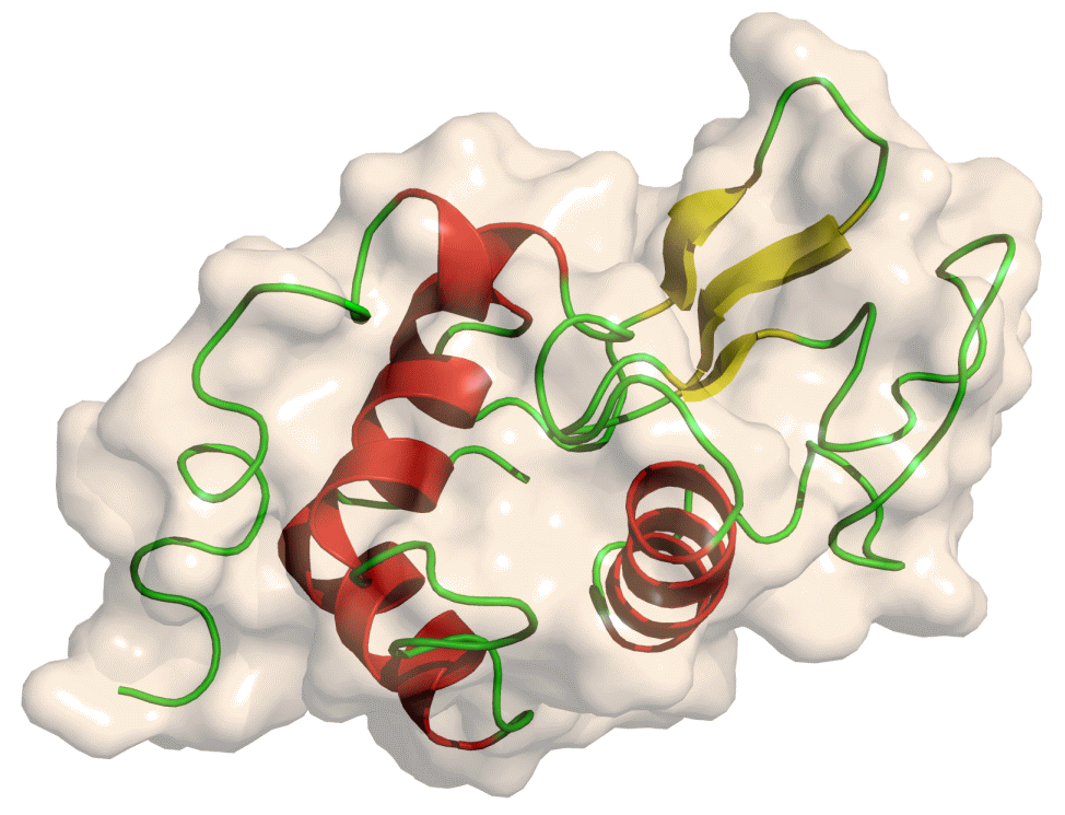 Open image in new tab
Setup
The GROMACS initial setup tool tool uses the PDB input to create three files which will be required for MD simulation.
Firstly, a topology for the protein structure is prepared. The topology file contains all the information required to describe the molecule for the purposes of simulation - atom masses, bond lengths and angles, charges. Note that this automatic construction of a topology is only possible if the building blocks of the molecules (i.e. amino acids in the case of a protein) are precalculated for the given force field. A force field and water model must be selected for topology calculation. Multiple choices are available for each; we will use the OPLS/AA force field and SPC/E water model. Secondly, a GRO structure file is created, storing the structure of the protein. Finally, a ‘position restraint file’ is created which will be used for NVT/NPT equilibration. We will return to this later.
In summary, the initial setup tool will:
- create a ‘topology’ file
- convert a PDB protein structure into a GRO file, with the structure centered in a simulation box (unit cell)
- create a position restraint file
After these files have been generated, a further step is required to define a simulation box (unit cell) in which the simulation can take place. This can be done with the GROMACS structure configuration tool tool. It also defines the unit cell ‘box’, centered on the structure. Options include box dimensions and shape; here, while a cuboidal box may be most intuitive, rhombic dodecahedron is the most efficient option, as it can contain the protein using the smallest volume, thus reducing the simulation resources devoted to the solvent.
Hands On: perform initial processing
- Run GROMACS initial setup ( Galaxy version 2020.4+galaxy0) with the following parameters:
- param-file “PDB input file”:
1AKI_clean.pdb(Input dataset)- “Water model”:
SPC/E- “Force field”:
OPLS/AA- “Ignore hydrogens”:
No- “Generate detailed log”:
YesQuestionWhy is it necessary to provide an input structure containing no non-protein molecules?
Automatic topology construction only succeeds if the components of the structure are recognized. For example, providing a structure of a protein in complex with a non-protein ligand or cofactor will result in an error.
- Run GROMACS structure configuration ( Galaxy version 2020.4+galaxy0) with the following parameters:
- “Input structure”: GRO output from initial setup tool
- “Output format”:
GRO file- “Configure box?”:
Yes- “Box dimensions in nanometers”:
1.0- “Box type”:
Rectangular box with all sides equal- “Generate detailed log”:
Yes
Solvation
The next stage is protein solvation, performed using GROMACS solvation and adding ions tool. Water molecules are added to the structure and topology files to fill the unit cell. At this stage sodium or chloride ions are also automatically added to neutralize the charge of the system. In our case, as lysozyme has a charge of +8, 8 chloride anions are added.
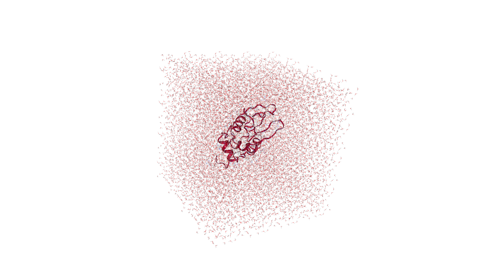 Open image in new tab
Hands On: solvationGROMACS solvation and adding ions ( Galaxy version 2020.4+galaxy1) with the following parameters:
- param-file “GRO structure file”: GRO structure file produced by the structure configuration tool
- param-file “Topology (TOP) file”: Topology produced by setup
- “Water model for solvation”:
SPC- “Add ions to neutralise system?”:
Yes, add ions- “Specify salt concentration (sodium chloride) to add, in mol/liter”:
0- “Generate detailed log”:
Yes
Energy minimization
To remove any steric clashes or unusual geometry which would artificially raise the energy of the system, we must relax the structure by running an energy minimization (EM) algorithm.
Here, and in the later steps, two options are presented under ‘Parameter input’. Firstly, the default setting, which we will use for this tutorial, requires options to be selected through the Galaxy interface. Alternatively, you can choose to upload an MDP (molecular dynamics parameters) file to define the simulation parameters. Using your own MDP file will allow greater customization, as not all parameters are implemented in Galaxy (yet); however, it requires a more advanced knowledge of GROMACS. Description of all parameters can be found here.
Hands On: energy minimizationGROMACS energy minimization ( Galaxy version 2020.4+galaxy0) with the following parameters:
- param-file “GRO structure file”: GRO structure file produced by solvation tool
- param-file “Topology (TOP) file”: Topology
- “Parameter input”:
Use default (partially customisable) setting- “Choice of integrator”:
Steepest descent algorithm(most common choice for EM)- “Neighbor searching”:
Generate a pair list with buffering(the ‘Verlet scheme’)- “Electrostatics”:
Fast smooth Particle-Mesh Ewald (SPME) electrostatics- “Distance for the Coulomb cut-off”:
1.0- “Cut-off distance for the short-range neighbor list”:
1.0(but irrelevant as we are using the Verlet scheme)- “Short range van der Waals cutoff”:
1.0- “Number of steps for the MD simulation”:
50000- “EM tolerance”:
1000- “Maximum step size”:
0.01- “Generate detailed log”:
Yes
Equilibration
At this point equilibration of the solvent around the solute (i.e. the protein) is necessary. This is performed in two stages: equilibration under an NVT ensemble, followed by an NPT ensemble. Use of the NVT ensemble entails maintaining constant number of particles, volume and temperature, while the NPT ensemble maintains constant number of particles, pressure and temperature. (The NVT ensemble is also known as the isothermal-isochoric ensemble, while the NPT ensemble is also known as the isothermal-isobaric ensemble).
During the first equilibration step (NVT), the protein must be held in place while the solvent is allowed to move freely around it. This is achieved using the position restraint file we created in system setup. When we specify this restraint, protein movement is not totally forbidden, but is energetically punished. During the second NPT step, we remove the restraints.
NVT equilibration
Firstly, we perform equilibration using classical NVT dynamics.
Hands On: NVT dynamicsGROMACS simulation ( Galaxy version 2020.4+galaxy1) with the following parameters:
- param-file “GRO structure file”: GRO structure file
- param-file “Topology (TOP) file”: Topology
- “Use a checkpoint (CPT) file”:
No CPT input- “Produce a checkpoint (CPT) file”:
Produce CPT output- “Apply position restraints”:
Apply position restraints- param-file “Position restraint file”: Position restraint file produced by ‘Setup’ tool.
- “Ensemble”:
Isothermal-isochoric ensemble (NVT).- “Trajectory output”:
Return no trajectory output(we are not interested in how the system evolves to the equilibrated state, merely the final structure)- “Structure output”:
Return .gro file- “Parameter input”:
Use default (partially customisable) setting- “Choice of integrator”:
A leap-frog algorithm for integrating Newton’s equations of motion(A basic leap-frog integrator)- “Bond constraints”:
Bonds with H-atoms(bonds involving H are constrained)- “Neighbor searching”:
Generate a pair list with buffering(the ‘Verlet scheme’)- “Electrostatics”:
Fast smooth Particle-Mesh Ewald (SPME) electrostatics- “Temperature”:
300- “Step length in ps”:
0.002- “Number of steps that elapse between saving data points (velocities, forces, energies)”:
5000- “Distance for the Coulomb cut-off”:
1.0- “Cut-off distance for the short-range neighbor list”:
1.0(but irrelevant as we are using the Verlet scheme)- “Short range van der Waals cutoff”:
1.0- “Number of steps for the NVT simulation”:
50000- “Generate detailed log”:
Yes
NPT equilibration
Having stabilized the temperature of the system with NVT equilibration, we also need to stabilize the pressure of the system. We therefore equilibrate again using the NPT (constant number of particles, pressure, temperature) ensemble.
Note that we can continue where the last simulation left off (with new parameters) by using the checkpoint (CPT) file saved at the end of the NVT simulation.
Hands On: NPT dynamicsGROMACS simulation ( Galaxy version 2020.4+galaxy1) with the following parameters:
- param-file “GRO structure file”: GRO structure file
- param-file “Topology (TOP) file”: Topology
- “Use a checkpoint (CPT) file”:
Continue simulation from a CPT file.- param-file “Checkpoint (CPT) file”: Checkpoint file produced by NVT equilibration
- “Produce a checkpoint (CPT) file”:
Produce CPT output- “Apply position restraints”:
No position restraints- param-file “Position restraint file”: None
- “Ensemble”:
Isothermal-isobaric ensemble (NPT).- “Trajectory output”:
Return no trajectory output- “Structure output”:
Return .gro file- “Parameter input”:
Use default (partially customisable) setting- “Choice of integrator”:
A leap-frog algorithm for integrating Newton’s equations of motion(A basic leap-frog integrator)- “Bond constraints”:
Bonds with H-atoms(bonds involving H are constrained)- “Neighbor searching”:
Generate a pair list with buffering(the ‘Verlet scheme’)- “Electrostatics”:
Fast smooth Particle-Mesh Ewald (SPME) electrostatics- “Temperature”:
300- “Step length in ps”:
0.002- “Number of steps that elapse between saving data points (velocities, forces, energies)”:
5000- “Distance for the Coulomb cut-off”:
1.0- “Cut-off distance for the short-range neighbor list”:
1.0(but irrelevant as we are using the Verlet scheme)- “Short range van der Waals cutoff”:
1.0- “Number of steps for the NPT simulation”:
50000- “Generate detailed log”:
Yes
QuestionWhy is the position of the protein restrained during equilibration?
The purpose of equilibration is to stabilize the temperature and pressure of the system; these are overwhelmingly dependent on the solvent. Structural changes in the protein are an additional complicating variable, which can more simply be removed by restraining the protein.
Production simulation
Now that equilibration is complete, we can release the position restraints. We are now finally ready to perform a production MD simulation.
Hands On: Production simulation
- GROMACS simulation ( Galaxy version 2020.4+galaxy1) with the following parameters:
- param-file “GRO structure file”: GRO structure file
- param-file “Topology (TOP) file”: Topology
- “Use a checkpoint (CPT) file”:
Continue simulation from a CPT file.- param-file “Checkpoint (CPT) file”: Checkpoint file produced by NPT equilibration
- “Produce a checkpoint (CPT) file”:
No CPT output- “Apply position restraints”:
No position restraints- “Ensemble”:
Isothermal-isobaric ensemble (NPT).- “Trajectory output”:
Return .xtc file (reduced precision)(this time, we save the trajectory)- “Structure output”:
Return .gro file- “Parameter input”:
Use default (partially customisable) setting- “Choice of integrator”:
A leap-frog algorithm for integrating Newton’s equations of motion(A basic leap-frog integrator)- “Bond constraints”:
Bonds with H-atoms(bonds involving H are constrained)- “Neighbor searching”:
Generate a pair list with buffering(the ‘Verlet scheme’)- “Electrostatics”:
Fast smooth Particle-Mesh Ewald (SPME) electrostatics- “Temperature”:
300- “Step length in ps”:
0.002- “Number of steps that elapse between saving data points (velocities, forces, energies)”:
5000- “Distance for the Coulomb cut-off”:
1.0- “Cut-off distance for the short-range neighbor list”:
1.0(but irrelevant as we are using the Verlet scheme)- “Short range van der Waals cutoff”:
1.0- “Number of steps for the simulation”:
500000- “Generate detailed log”:
Yes
Workflow
A GROMACS workflow is provided for this tutorial. Overall, the workflow takes a PDB (Protein Data Bank) structure file as input and returns a MD trajectory.
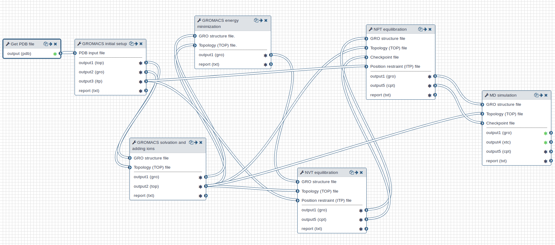 Open image in new tab
Conclusion
After completing the steps, or running the workflow, we have successfully produced a trajectory (the xtc file) which describes the atomic motion of the system. This can be viewed using molecular visualization software or analysed further; please visit the visualization and analysis tutorials for more information.
 Open image in new tab
You've Finished the Tutorial
Key points
Molecular dynamics produces a trajectory describing the atomic motion of a system.
Preparation of the system is required; setup, solvation, minimization, equilibration.
Frequently Asked Questions
Have questions about this tutorial? Have a look at the available FAQ pages and support channelsUseful literature
Further information, including links to documentation and original publications, regarding the tools, analysis techniques and the interpretation of results described in this tutorial can be found here.
References
- Abraham, M. J., T. Murtola, R. Schulz, S. Páll, J. C. Smith et al., 2015 GROMACS: High performance molecular simulations through multi-level parallelism from laptops to supercomputers. SoftwareX 1-2: 19–25. https://doi.org/10.1016/j.softx.2015.06.001 http://www.sciencedirect.com/science/article/pii/S2352711015000059
Feedback
Did you use this material as an instructor? Feel free to give us feedback on how it went.
Did you use this material as a learner or student? Click the form below to leave feedback.

Citing this Tutorial
- Simon Bray, Running molecular dynamics simulations using GROMACS (Galaxy Training Materials). https://training.galaxyproject.org/training-material/topics/computational-chemistry/tutorials/md-simulation-gromacs/tutorial.html Online; accessed TODAY
- Hiltemann, Saskia, Rasche, Helena et al., 2023 Galaxy Training: A Powerful Framework for Teaching! PLOS Computational Biology 10.1371/journal.pcbi.1010752
- Batut et al., 2018 Community-Driven Data Analysis Training for Biology Cell Systems 10.1016/j.cels.2018.05.012
Congratulations on successfully completing this tutorial!@misc{computational-chemistry-md-simulation-gromacs, author = "Simon Bray", title = "Running molecular dynamics simulations using GROMACS (Galaxy Training Materials)", year = "", month = "", day = "", url = "\url{https://training.galaxyproject.org/training-material/topics/computational-chemistry/tutorials/md-simulation-gromacs/tutorial.html}", note = "[Online; accessed TODAY]" } @article{Hiltemann_2023, doi = {10.1371/journal.pcbi.1010752}, url = {https://doi.org/10.1371%2Fjournal.pcbi.1010752}, year = 2023, month = {jan}, publisher = {Public Library of Science ({PLoS})}, volume = {19}, number = {1}, pages = {e1010752}, author = {Saskia Hiltemann and Helena Rasche and Simon Gladman and Hans-Rudolf Hotz and Delphine Larivi{\`{e}}re and Daniel Blankenberg and Pratik D. Jagtap and Thomas Wollmann and Anthony Bretaudeau and Nadia Gou{\'{e}} and Timothy J. Griffin and Coline Royaux and Yvan Le Bras and Subina Mehta and Anna Syme and Frederik Coppens and Bert Droesbeke and Nicola Soranzo and Wendi Bacon and Fotis Psomopoulos and Crist{\'{o}}bal Gallardo-Alba and John Davis and Melanie Christine Föll and Matthias Fahrner and Maria A. Doyle and Beatriz Serrano-Solano and Anne Claire Fouilloux and Peter van Heusden and Wolfgang Maier and Dave Clements and Florian Heyl and Björn Grüning and B{\'{e}}r{\'{e}}nice Batut and}, editor = {Francis Ouellette}, title = {Galaxy Training: A powerful framework for teaching!}, journal = {PLoS Comput Biol} }
Do you want to extend your knowledge?Follow one of our recommended follow-up trainings:
You can use Ephemeris's
shed-tools installcommand to install the tools used in this tutorial.shed-tools install [-g GALAXY] [-a API_KEY] -t <(curl https://training.galaxyproject.org/training-material/api/topics/computational-chemistry/tutorials/md-simulation-gromacs/tutorial.json | jq .admin_install_yaml -r)Alternatively you can copy and paste the following YAML
---
install_tool_dependencies: true
install_repository_dependencies: true
install_resolver_dependencies: true
tools:
- name: get_pdb
  owner: bgruening
  revisions: 538790c6c21b
  tool_panel_section_label: ChemicalToolBox
  tool_shed_url: https://toolshed.g2.bx.psu.edu/
- name: text_processing
  owner: bgruening
  revisions: d698c222f354
  tool_panel_section_label: Text Manipulation
  tool_shed_url: https://toolshed.g2.bx.psu.edu/
- name: gmx_editconf
  owner: chemteam
  revisions: bfb65cb551d8
  tool_panel_section_label: ChemicalToolBox
  tool_shed_url: https://toolshed.g2.bx.psu.edu/
- name: gmx_editconf
  owner: chemteam
  revisions: 0fac8e2afc13
  tool_panel_section_label: ChemicalToolBox
  tool_shed_url: https://toolshed.g2.bx.psu.edu/
- name: gmx_em
  owner: chemteam
  revisions: 55918daa5651
  tool_panel_section_label: ChemicalToolBox
  tool_shed_url: https://toolshed.g2.bx.psu.edu/
- name: gmx_em
  owner: chemteam
  revisions: f5d979cb4b54
  tool_panel_section_label: ChemicalToolBox
  tool_shed_url: https://toolshed.g2.bx.psu.edu/
- name: gmx_setup
  owner: chemteam
  revisions: 4da9ee404eab
  tool_panel_section_label: ChemicalToolBox
  tool_shed_url: https://toolshed.g2.bx.psu.edu/
- name: gmx_setup
  owner: chemteam
  revisions: 2c349b027a01
  tool_panel_section_label: ChemicalToolBox
  tool_shed_url: https://toolshed.g2.bx.psu.edu/
- name: gmx_sim
  owner: chemteam
  revisions: f197e34c33a9
  tool_panel_section_label: ChemicalToolBox
  tool_shed_url: https://toolshed.g2.bx.psu.edu/
- name: gmx_sim
  owner: chemteam
  revisions: 73008ef1f487
  tool_panel_section_label: ChemicalToolBox
  tool_shed_url: https://toolshed.g2.bx.psu.edu/
- name: gmx_solvate
  owner: chemteam
  revisions: 27ea4e1a3f95
  tool_panel_section_label: ChemicalToolBox
  tool_shed_url: https://toolshed.g2.bx.psu.edu/
- name: gmx_solvate
  owner: chemteam
  revisions: 2c8ed1b52bf7
  tool_panel_section_label: ChemicalToolBox
  tool_shed_url: https://toolshed.g2.bx.psu.edu/