Genome Assembly of MRSA from Oxford Nanopore MinION data (and optionally Illumina data)
| Author(s) |
|
| Editor(s) |
|
| Reviewers |
|
OverviewQuestions:
Objectives:
How to check the quality of the MinION data (together with Illumina data)?
How to perform an assembly of a bacterial genome with MinION data?
How to check the quality of an assembly?
Requirements:
Run tools to evaluate sequencing data on quality and quantity
Process the output of quality control tools
Improve the quality of sequencing data
Run a tool to assemble a bacterial genome using short reads
Run tools to assess the quality of an assembly
Understand the outputs of tools to assess the quality of an assembly
Time estimation: 2 hoursLevel: Introductory IntroductorySupporting Materials:Published: Mar 24, 2021Last modification: Jan 5, 2026License: Tutorial Content is licensed under Creative Commons Attribution 4.0 International License. The GTN Framework is licensed under MITpurl PURL: https://gxy.io/GTN:T00037rating Rating: 3.7 (3 recent ratings, 7 all time)version Revision: 16
Sequencing (determining of DNA/RNA nucleotide sequence) is used all over the world for all kinds of analysis. The product of these sequencers are reads, which are sequences of detected nucleotides. Depending on the technique these have specific lengths (30-500bp) or using Oxford Nanopore Technologies sequencing have much longer variable lengths.
Comment: Nanopore sequencingNanopore sequencing has several properties that make it well-suited for our purposes
- Long-read sequencing technology offers simplified and less ambiguous genome assembly
- Long-read sequencing gives the ability to span repetitive genomic regions
- Long-read sequencing makes it possible to identify large structural variations
")
When using Oxford Nanopore Technologies (ONT) sequencing, the change in electrical current is measured over the membrane of a flow cell. When nucleotides pass the pores in the flow cell the current change is translated (basecalled) to nucleotides by a basecaller. A schematic overview is given in the picture above.
When sequencing using a MinIT or MinION Mk1C, the basecalling software is present on the devices. With basecalling the electrical signals are translated to bases (A,T,G,C) with a quality score per base. The sequenced DNA strand will be basecalled and this will form one read. Multiple reads will be stored in a fastq file.
In this training we will build an assembly of a bacterial genome, from data produced in “Complete Genome Sequences of Eight Methicillin-Resistant Staphylococcus aureus Strains Isolated from Patients in Japan” Hikichi et al. 2019:
Methicillin-resistant Staphylococcus aureus (MRSA) is a major pathogen causing nosocomial infections, and the clinical manifestations of MRSA range from asymptomatic colonization of the nasal mucosa to soft tissue infection to fulminant invasive disease. Here, we report the complete genome sequences of eight MRSA strains isolated from patients in Japan.
AgendaIn this tutorial, we will cover:
Galaxy and data preparation
Any analysis should get its own Galaxy history. So let’s start by creating a new one and get the data into it.
Hands On: History creation
Create a new history for this analysis
To create a new history simply click the new-history icon at the top of the history panel:
Rename the history
- Click on galaxy-pencil (Edit) next to the history name (which by default is “Unnamed history”)
- Type the new name
- Click on Save
- To cancel renaming, click the galaxy-undo “Cancel” button
If you do not have the galaxy-pencil (Edit) next to the history name (which can be the case if you are using an older version of Galaxy) do the following:
- Click on Unnamed history (or the current name of the history) (Click to rename history) at the top of your history panel
- Type the new name
- Press Enter

Now, we need to import the data: 1 FASTQ file containing the reads from the sequencer.
Hands On: Data upload
Import the files from Zenodo or from the shared data library
https://zenodo.org/record/10669812/files/DRR187567.fastq.bz2
- Copy the link location
Click galaxy-upload Upload at the top of the activity panel
- Select galaxy-wf-edit Paste/Fetch Data
Paste the link(s) into the text field
Press Start
- Close the window
As an alternative to uploading the data from a URL or your computer, the files may also have been made available from a shared data library:
- Go into Libraries (left panel)
- Navigate to the correct folder as indicated by your instructor.
- On most Galaxies tutorial data will be provided in a folder named GTN - Material –> Topic Name -> Tutorial Name.
- Select the desired files
- Click on Add to History galaxy-dropdown near the top and select as Datasets from the dropdown menu
In the pop-up window, choose
- “Select history”: the history you want to import the data to (or create a new one)
- Click on Import
Rename the dataset to keep only the sequence run ID (
DRR187567)
- Click on the galaxy-pencil pencil icon for the dataset to edit its attributes
- In the central panel, change the Name field to
DRR187567- Click the Save button
Tag the dataset
#unfilteredDatasets can be tagged. This simplifies the tracking of datasets across the Galaxy interface. Tags can contain any combination of letters or numbers but cannot contain spaces.
To tag a dataset:
- Click on the dataset to expand it
- Click on Add Tags galaxy-tags
- Add tag text. Tags starting with
#will be automatically propagated to the outputs of tools using this dataset (see below).- Press Enter
- Check that the tag appears below the dataset name
Tags beginning with
#are special!They are called Name tags. The unique feature of these tags is that they propagate: if a dataset is labelled with a name tag, all derivatives (children) of this dataset will automatically inherit this tag (see below). The figure below explains why this is so useful. Consider the following analysis (numbers in parenthesis correspond to dataset numbers in the figure below):
- a set of forward and reverse reads (datasets 1 and 2) is mapped against a reference using Bowtie2 generating dataset 3;
- dataset 3 is used to calculate read coverage using BedTools Genome Coverage separately for
+and-strands. This generates two datasets (4 and 5 for plus and minus, respectively);- datasets 4 and 5 are used as inputs to Macs2 broadCall datasets generating datasets 6 and 8;
- datasets 6 and 8 are intersected with coordinates of genes (dataset 9) using BedTools Intersect generating datasets 10 and 11.
Now consider that this analysis is done without name tags. This is shown on the left side of the figure. It is hard to trace which datasets contain “plus” data versus “minus” data. For example, does dataset 10 contain “plus” data or “minus” data? Probably “minus” but are you sure? In the case of a small history like the one shown here, it is possible to trace this manually but as the size of a history grows it will become very challenging.
The right side of the figure shows exactly the same analysis, but using name tags. When the analysis was conducted datasets 4 and 5 were tagged with
#plusand#minus, respectively. When they were used as inputs to Macs2 resulting datasets 6 and 8 automatically inherited them and so on… As a result it is straightforward to trace both branches (plus and minus) of this analysis.More information is in a dedicated #nametag tutorial.
View galaxy-eye the renamed file


The dataset is a FASTQ file.
Question
- What are the 4 main features of each read in a fastq file.
- What is the name of your first read?
The following:
- A
@followed by a name and sometimes information of the read- A nucleotide sequence
- A
+(optional followed by the name)- The quality score per base of nucleotide sequence (Each symbol represents a quality score, which will be explained later)
DRR187567.1
Hands-on: Choose Your Own TutorialThis is a 'Choose Your Own Tutorial' (CYOT) section (also known as 'Choose Your Own Analysis' (CYOA)), where you can select between multiple paths. Click one of the buttons below to select how you want to follow the tutorial
Do you have associated Illumina MiSeq data?
Hands On: Illumina Data upload
Import the files from Zenodo or from the shared data library
https://zenodo.org/record/10669812/files/DRR187559_1.fastqsanger.bz2
https://zenodo.org/record/10669812/files/DRR187559_2.fastqsanger.bz2
- Copy the link location
Click galaxy-upload Upload at the top of the activity panel
- Select galaxy-wf-edit Paste/Fetch Data
Paste the link(s) into the text field
Press Start
- Close the window
As an alternative to uploading the data from a URL or your computer, the files may also have been made available from a shared data library:
- Go into Libraries (left panel)
- Navigate to the correct folder as indicated by your instructor.
- On most Galaxies tutorial data will be provided in a folder named GTN - Material –> Topic Name -> Tutorial Name.
- Select the desired files
- Click on Add to History galaxy-dropdown near the top and select as Datasets from the dropdown menu
In the pop-up window, choose
- “Select history”: the history you want to import the data to (or create a new one)
- Click on Import
Rename the datasets to remove
.fastqsanger.bz2and keep only the sequence run ID (DRR187559_1andDRR187559_2)
- Click on the galaxy-pencil pencil icon for the dataset to edit its attributes
- In the central panel, change the Name field to
DRR187567- Click the Save button
Create a paired collection named
Paired Reads
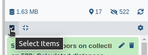
- Click on galaxy-selector Select Items at the top of the history panel
- Check all the datasets in your history you would like to include
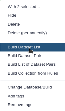
Click n of N selected and choose Advanced Build List
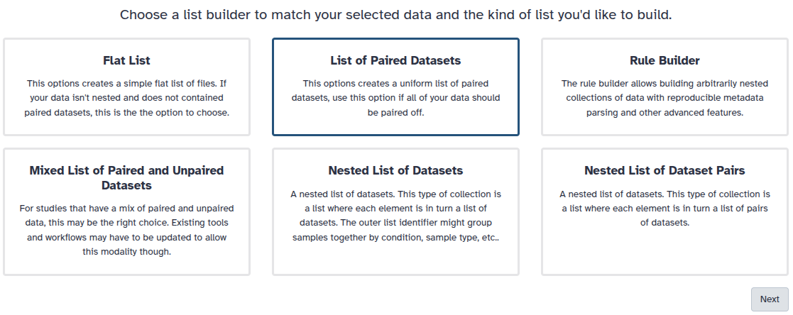
You are in the collection building wizard. Choose List of Paired Datasets and click ‘Next’ button at the right bottom corner.
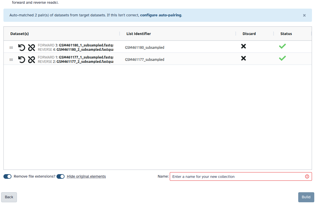
Check and configure auto-pairing. Commonly matepairs have suffix
_1and_2or_R1and_R2. Click on ‘Next’ at the bottom.
- Edit the List Identifier as required.
- Enter a name for your collection
- Click Build to build your collection
- Click on the checkmark icon at the top of your history again
Quality Control
During sequencing, errors are introduced, such as incorrect nucleotides being called. These are due to the technical limitations of each sequencing platform. Sequencing errors might bias the analysis and can lead to a misinterpretation of the data. Sequence quality control is therefore an essential first step in any analysis.
When assessing the fastq files all bases had their own quality (or Phred score) represented by symbols. You can read more in our dedicated Quality Control Tutorial.
To assess the quality by hand would be too much work. That’s why tools like NanoPlot or FastQC are made, which will generate a summary and plots of the data statistics. NanoPlot is mainly used for long-read data, like ONT and PACBIO and FastQC for any read.
Hands On: Quality Control
- FastQC ( Galaxy version 0.74+galaxy0) with the following parameters:
- param-files “Short read data from your current history”:
DRR187567- Inspect the webpage output
FastQC combines quality statistics from all separate reads and combines them in plots. An important plot is the Per base sequence quality.
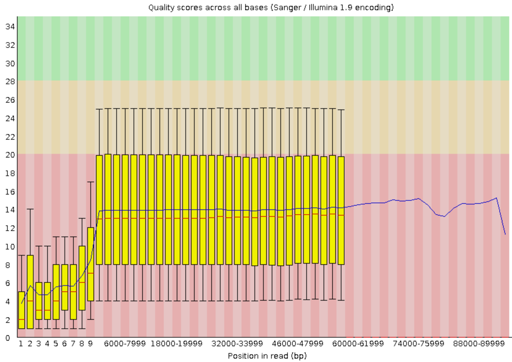
Here, we are going to trim the Illumina data using fastp (Chen et al. 2018):
- Trim the start and end of the reads if those fall below a quality score of 20
- Filter for reads to keep only reads with at least 30 bases: Anything shorter will complicate the assembly
Hands On: Quality improvement of the Illumina reads
- fastp ( Galaxy version 1.0.1+galaxy3) with the following parameters:
- “Single-end or paired reads”:
Paired Collection
- “Select paired collection(s)”:
Paired Reads- In “Filter Options”:
- In “Length filtering Options”:
- Length required:
30- In “Read Modification Options”:
- In “Per read cuitting by quality options”:
- Cut by quality in front (5’):
Yes- Cut by quality in tail (3’):
Yes- Cutting window size:
4- Cutting mean quality:
20- In “Output Options”:
- “Output JSON report”:
YesWe next need to extract the fastp filtered forward and reverse reads from the paired collection as the next tool we are going to run, filtlong, requires the forward and reverse short reads to be provided as separate datasets.
- Flatten collection with the following parameters:
- “Input Collection”: fastp
Paired-end outputRename galaxy-pencil the output to
Flattened fastp output- Extract dataset with the following parameters:
- “Input List”:
Flattened fastp output- “How should a dataset be selected?”:
Select by element identifier- “Element identifier”:
DRR187559_forward(filtered forward reads)Rename galaxy-pencil
DRR187559_forwardtoTrimmed DRR187559_forward- Extract dataset with the following parameters:
- “Input List”:
Flattened fastp output- “How should a dataset be selected?”:
Select by element identifier- “Element identifier”:
DRR187559_reverse(filtered forward reads)- Rename galaxy-pencil
DRR187559_reversetoTrimmed DRR187559_reverse
Depending on the analysis it could be possible that a certain quality or length is needed. The reads can be filtered using the Filtlong tool. In this training all reads below 1000bp will be filtered.
When Illumina reads are available, we can use them if they are good Illumina reads (high depth and complete coverage) as external reference. In this case, Filtlong ignores the Phred quality scores and instead judges read quality using k-mer matches to the reference (a more accurate gauge of quality).
Hands On: Filtering
- filtlong ( Galaxy version 0.2.1+galaxy0) with the following parameters:
- param-file “Input FASTQ”:
DRR187567- In “Output thresholds”:
- “Min. length”:
1000
- In “External references”:
- param-file “Reference Illumina read”:
Trimmed DRR187559_forward- param-file “Reference Illumina read”:
Trimmed DRR187559_reverseRename the dataset to
DRR187567-filtered
- Click on the galaxy-pencil pencil icon for the dataset to edit its attributes
- In the central panel, change the Name field to
DRR187567-filtered- Click the Save button
The output can be evaluated using NanoPlot for plotting long read sequencing data and alignments
Hands On: Filtering
Convert the datatype of
DRR187567to uncompress it
- Click on the galaxy-pencil pencil icon for the dataset to edit its attributes.
- In the central panel, click galaxy-chart-select-data Datatypes tab on the top.
- In the galaxy-gear Convert to Datatype section, select
Convert compressed to uncompressedfrom “Target datatype” dropdown.- Click the Create Dataset button to start the conversion.
NanoPlot ( Galaxy version 1.41.0+galaxy0) with the following parameters:
- “Select multifile mode”:
batch
- “Type of the file(s) to work on”:
fastq
- param-files “files”: both
DRR187567 uncompressedandDRR187567-filtered- In “Options for customizing the plots created”:
- “Show the N50 mark in the read length histogram.”:
Yes
We ran the NanoPlot two times: one for the raw reads (DRR187567) and one for the reads after filtering (DRR187567-filtered).
For each run, NanoPlot generates 5 outputs:
- 2 plots:
- Histogram Read Length
-
Histogram Read Length after log transformation
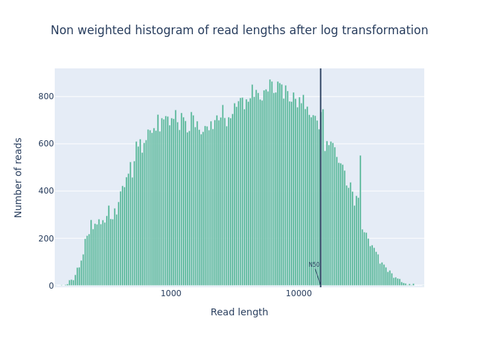 Open image in new tab
Figure 1: Before filtering 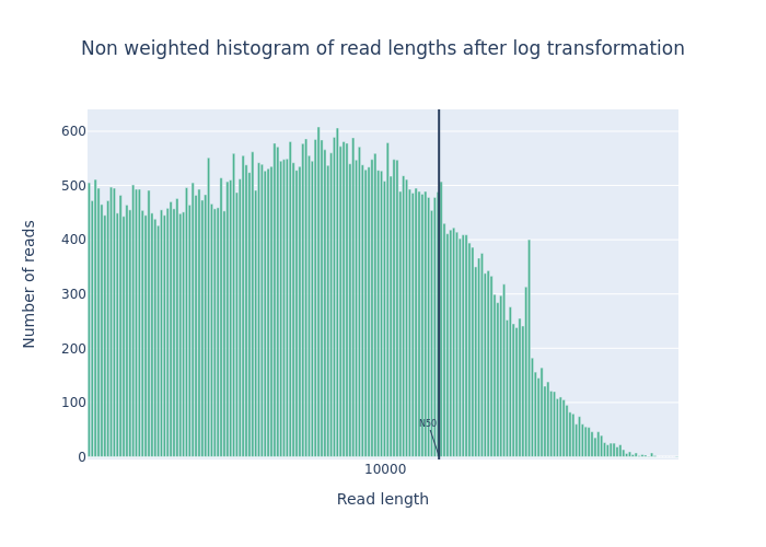 Open image in new tab
Figure 2: After filtering
-
2 tabular files with statistics: one general and one after filtering.
The second one is empty because we did not used NanoPlot filtering options.
-
A HTML report summarizing above information
We can compare the two generated reports. Galaxy allows to view several datasets side-by-side using the Window Manager function
Hands On: Inspect NanoPlot reports-
Enable Window Manager
If you would like to view two or more datasets at once, you can use the Window Manager feature in Galaxy:
- Click on the Window Manager icon galaxy-scratchbook on the top menu bar.
- You should see a little checkmark on the icon now
- View galaxy-eye a dataset by clicking on the eye icon galaxy-eye to view the output
- You should see the output in a window overlayed over Galaxy
- You can resize this window by dragging the bottom-right corner
- View galaxy-eye a second dataset from your history
- You should now see a second window with the new dataset
- This makes it easier to compare the two outputs
- Repeat this for as many files as you would like to compare
- You can turn off the Window Manager galaxy-scratchbook by clicking on the icon again
- Click on the Window Manager icon galaxy-scratchbook on the top menu bar.
- Open both NanoPlot HTML Reports
- Check the Summary statistics section of each to compare the results
Summary statistics Not Filtered Filtered (Filtlong) Change (%) Number of reads 91,288 69,906 -23.4% Number of bases 621,945,741.0 609,657,642.0 -2.0% Median read length 3,400.0 5,451.0 60.3% Mean read length 6,813.0 8,721.1 28.0% Read length N50 14,810.0 15,102.0 2.0% Mean read quality 9 9 0.0% Median read quality 8.9 9.0 1.1% Question- What is the increase of your median read length?
- What is the decrease in the number of bases?
- What is coverage?
- What would be the coverage before and after trimming, based on a genome size of 2.9 Mbp?
- 3,400 bp to 5,451 bp, a 60.3% increase
- A -2.0% decrease is not a very significant decrease. Our data was quite good to start with and didn’t have many short reads which were removed (23.4%)
- The coverage is a measure of how many reads ‘cover’ on average a single base in the genome. If you divide the total reads by the genome size, you will get a number how many times your genomes could theoretically be “covered” by reads.
- Before \(\frac{621,945,741}{2,900,000} = 214.4\) and after \(\frac{609,657,642}{2,900,000} = 210.2\). This is not a very big decrease in coverage, so no cause for concern. Generally in sequencing experiments you have some minimum coverage you expect to see based on how much of your sample you sequenced. If it falls below that threshold it might be cause for concern.
-
While there is currently no community consensus over the best trimming or filtering practices with long read data, there are still some steps that can be beneficial to do for the assembly process. Porechop ( Galaxy version 0.2.3) is a commonly used tool for removing adapter sequences, and we used filtlong ( Galaxy version 0.2.0) for removing shorter reads which might make the assembly process more difficult.
Many people do not do any trimming of their NanoPore data based on the quality as it is expected that the quality is low, and often the focus is on assembling large Structural Variations (SVs) rather than having high quality reads and base-level variation analyses.
Assembly
When the quality of the reads is determined and the data is filtered (like we did with filtlong) and/or trimmed (like is more often done with short read data) an assembly can be made.
There are many tools that create assembly for long-read data, e.g. Canu (Koren et al. 2017), Raven (Vaser and Šikić 2021), Miniasm (Li 2016). In this tutorial, we use Flye (Lin et al. 2016). Flye is a de novo assembler for single molecule sequencing reads. It can be used from bacteria to human assemblies. The Flye assembly is based on finding overlapping reads with variable length with high error tolerance.
Comment: Results may varyYour results may be slightly different from the ones presented in this tutorial due to differing versions of tools, reference data, external databases, or because of stochastic processes in the algorithms.
Hands On: Assembly using Flye
- Flye assembly ( Galaxy version 2.9.1+galaxy0) with the following parameters:
- param-file “Input reads”:
DRR187567-filtered(output of filtlong tool)- “Mode”:
Nanopore corrected (--nano-corr)- “Reduced contig assembly coverage”:
Disable reduced coverage for initial disjointing assembly
Flye generates 4 outputs:
-
A FASTA file called
consensuswith contigs, i.e. the contiguous sequences made by combining separate reads in the assembly, and possibly scaffolds built by FlyeQuestionHow many contigs are there?
There are 2 sequences in the
consensusdataset -
2 assembly graph files:
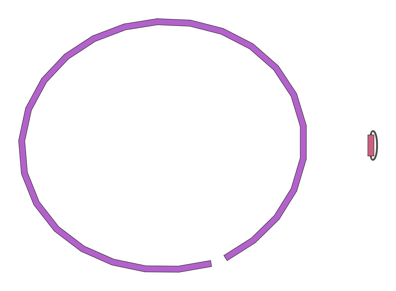
assembly graphandgraphical fragment assemblyWe can visualize the assembly graph using the
graphical fragment assemblywith Bandage (Wick et al. 2015), a package for exploring assembly graphs through summary reports and visualizations of their contents.Hands On: Assembly inspection- Bandage Image ( Galaxy version 2022.09+galaxy4) with the following parameters:
- param-file “Graphical Fragment Assembly”:
graphical fragment assembly(output of Flye)
- param-file “Graphical Fragment Assembly”:
- Bandage Image ( Galaxy version 2022.09+galaxy4) with the following parameters:
-
A table
assembly infowith assembly informationIt should be something similar but probably sligtly different because Flye can differ a bit per assembly:
#seq_name length cov. circ. repeat mult. alt_group graph_path contig_1 2927029 183 Y N 2 * 1 contig_2 60115 379 Y Y 2 * 2 Question- What is the coverage of your longest contig?
- What is the length of your longest contig?
- Could this contig potentially be a MRSA genome?
While results may vary due to randomness in the assembly process, in our case we had:
- 183
- 2.9Mb
- 2.9Mb is approximately the size of a MRSA genome. So contig 1 could be the genome. Contig 2 could be one small potential plasmid genome.
Assembly Evaluation
To evaluate the assembly, we use also Quast (Gurevich et al. 2013) (QUality ASsessment Tool), a tool providing quality metrics for assemblies. This tool can be used to compare multiple assemblies, can take an optional reference file as input to provide complementary metrics, etc
Hands On: Quality Control of assembly using Quast
- Quast ( Galaxy version 5.2.0+galaxy1) with the following parameters:
- Assembly mode?:
Co-assembly
- “Use customized names for the input files?”:
No, use dataset names
- param-file “Contigs/scaffolds file”:
consensusoutput of Flye
QUAST outputs assembly metrics as an HTML file with metrics and graphs.
Question
- How many contigs is there?
- How long is the largest contig?
- What is the total length of all contigs?
- What is you GC content?
- How does it compare to results for KUN1163 in Table 1 in Hikichi et al. 2019?
- 2 contigs
- The largest contig is 2,907,099 bp.
- 2,967,214 (Total length (>= 0 bp)).
- The GC content for our assembly is 32.91%.
- KUN1163 has a genome size of 2,914,567 bp (not far from the length of the largest contig), with a GC content of 32.91% (as in our assembly)
Assembly Polishing
We can now polish the assembly using both the short reads and/or long reads. This process aligns the reads to the assembly contigs, and makes corrections to the contigs where warranted.
Several tools exist for polishing, e.g. Racon (Vaser et al. 2017). Here we will use Polypolish (Wick and Holt 2022), a tool for polishing genome assemblies with short reads.
Polypolish needs as input the assembly but also SAM/BAM files where each read has been aligned to all possible locations (not just a single best location). Errors in repeats will be covered by short-read alignments, and Polypolish can therefore fix those errors.
To get the SAM/BAM files, we need to map the short reads on the assembly. We will use BWA-MEM (Li and Durbin 2009, Li and Durbin 2010, Li 2013).
We need to set up BWA-MEM so it aligns each read to all possible locations, not just the best location. This option does not work with paired-end alignment. We will then need to align forward and reverse read files separately, instead of aligning both read files with a single BWA-MEM run as usually recommended.
Hands On: Align short-reads on assembly
Change the datatype of both FASTQ outputs of fastp to
fastqsanger.gz
- Click on the galaxy-pencil pencil icon for the dataset to edit its attributes
- In the central panel, click galaxy-chart-select-data Datatypes tab on the top
- In the galaxy-chart-select-data Assign Datatype, select
fastqsanger.gzfrom “New Type” dropdown
- Tip: you can start typing the datatype into the field to filter the dropdown menu
- Click the Save button
BWA-MEM2 ( Galaxy version 2.2.1+galaxy1) with the following parameters:
- “Will you select a reference genome from your history or use a built-in index?”:
Use a genome from history and build index
- param-file “Use the following dataset as the reference sequence”:
consensusoutput of Flye- “Single or Paired-end reads”:
Single
- param-files “Select fastq dataset”:
DRR187559_forward,DRR187559_reverse- “Set read groups information?”:
Do not set- “Select analysis mode”:
5.Full list of options
- “Set algorithmic options?”:
Do not set- “Set scoring options?”:
Do not set- “Set input/output options”:
Set
- “Output all alignments for single-ends or unpaired paired-ends”:
Yes- “BAM sorting mode”:
Not sorted (sorted as input)
We can now run Polypolish.
Hands On: Polish assembly
- Polypolish ( Galaxy version 0.5.0+galaxy2) with the following parameters:
- In “Input sequences”:
- param-file “Select a draft genome for polishing”:
consensusoutput of Flye- “Select aligned data to polish”:
Paired SAM/BAM files
- param-file “Select forward SAM/BAM file”: output of BWA-MEM2 on the
DRR187559_forwardoutput of fastp- param-file “Select reverse SAM/BAM file”: output of BWA-MEM2 on the
DRR187559_reverseoutput of fastp
To check the impact of the polishing, let’s run QUAST on both Flye and Polypolish outputs.
Hands On: Quality Control of polished assembly
- Quast ( Galaxy version 5.2.0+galaxy1) with the following parameters:
- Assembly mode?:
Co-assembly
- “Use customized names for the input files?”:
No, use dataset names
- param-files “Contigs/scaffolds file”:
consensusoutput of Flye and output of Polypolish
The HTML report generated by QUAST gives metrics for both assembly side-by-side
| Statistics | Flye output | Polypolish output |
|---|---|---|
| Number of contigs | 2 | 2 |
| Largest contig | 2,907,099 | 2,915,230 |
| Total length (>= 0 bp) | 2,967,214 | 2,975,666 |
| GC (%) | 32.91 | 32.84 |
QuestionIs the assembly after polishing better than before given the results for KUN1163 in Table 1 in Hikichi et al. 2019?
The largest contig after polishing has a length of 2,915,230 bp, which closr to the expected 2,914,567 bp. But the GC content (32.84% after polishing) is slightly worst given the expected 32.91% also found in the assembly before polishing.
Conclusion
In this tutorial, we prepared long reads (using short reads if we had some) assembled them, inspect the produced assembly for its quality, and polished it (if short reads where provided). The assembly, even if uncomplete, is reasonable good to be used in downstream analysis, like AMR gene detection
You've Finished the Tutorial
Key points
Nanopore produces fantastic assemblies but with low quality data
Annotation with Prokka is very easy
Frequently Asked Questions
Have questions about this tutorial? Have a look at the available FAQ pages and support channelsReferences
- Li, H., and R. Durbin, 2009 Fast and accurate short read alignment with Burrows-Wheeler transform. Bioinformatics 25: 1754–1760. 10.1093/bioinformatics/btp324
- Li, H., and R. Durbin, 2010 Fast and accurate long-read alignment with Burrows–Wheeler transform. Bioinformatics 26: 589–595. 10.1093/bioinformatics/btp698
- Gurevich, A., V. Saveliev, N. Vyahhi, and G. Tesler, 2013 QUAST: quality assessment tool for genome assemblies. Bioinformatics 29: 1072–1075. 10.1093/bioinformatics/btt086
- Li, H., 2013 Aligning sequence reads, clone sequences and assembly contigs with BWA-MEM. 10.48550/arXiv.1303.3997
- Wick, R. R., M. B. Schultz, J. Zobel, and K. E. Holt, 2015 Bandage: interactive visualization of de novo genome assemblies. Bioinformatics 31: 3350–3352. 10.1093/bioinformatics/btv383
- Li, H., 2016 Minimap and miniasm: fast mapping and de novo assembly for noisy long sequences. Bioinformatics 32: 2103–2110. 10.1093/bioinformatics/btw152
- Lin, Y., J. Yuan, M. Kolmogorov, M. W. Shen, M. Chaisson et al., 2016 Assembly of long error-prone reads using de Bruijn graphs. Proceedings of the National Academy of Sciences 113: E8396–E8405. 10.1073/pnas.1604560113
- Koren, S., B. P. Walenz, K. Berlin, J. R. Miller, N. H. Bergman et al., 2017 Canu: scalable and accurate long-read assembly via adaptive k-mer weighting and repeat separation. Genome research 27: 722–736. 10.1101/gr.215087.116
- Vaser, R., I. Sović, N. Nagarajan, and M. Šikić, 2017 Fast and accurate de novo genome assembly from long uncorrected reads. Genome Research 27: 737–746. 10.1101/gr.214270.116
- Chen, S., Y. Zhou, Y. Chen, and J. Gu, 2018 fastp: an ultra-fast all-in-one FASTQ preprocessor. 10.1093/bioinformatics/bty560
- Hikichi, M., M. Nagao, K. Murase, C. Aikawa, T. Nozawa et al., 2019 Complete Genome Sequences of Eight Methicillin-Resistant Staphylococcus aureus Strains Isolated from Patients in Japan (I. L. G. Newton, Ed.). Microbiology Resource Announcements 8: 10.1128/mra.01212-19
- Vaser, R., and M. Šikić, 2021 Time-and memory-efficient genome assembly with Raven. Nature Computational Science 1: 332–336. 10.1038/s43588-021-00073-4
- Wick, R. R., and K. E. Holt, 2022 Polypolish: Short-read polishing of long-read bacterial genome assemblies (D. Schneidman-Duhovny, Ed.). PLOS Computational Biology 18: e1009802. 10.1371/journal.pcbi.1009802
Glossary
- SVs
- Structural Variations
Feedback
Did you use this material as an instructor? Feel free to give us feedback on how it went.
Did you use this material as a learner or student? Click the form below to leave feedback.

Citing this Tutorial
- Bazante Sanders, Bérénice Batut, Genome Assembly of MRSA from Oxford Nanopore MinION data (and optionally Illumina data) (Galaxy Training Materials). https://training.galaxyproject.org/training-material/topics/assembly/tutorials/mrsa-nanopore/tutorial.html Online; accessed TODAY
- Hiltemann, Saskia, Rasche, Helena et al., 2023 Galaxy Training: A Powerful Framework for Teaching! PLOS Computational Biology 10.1371/journal.pcbi.1010752
- Batut et al., 2018 Community-Driven Data Analysis Training for Biology Cell Systems 10.1016/j.cels.2018.05.012
@misc{assembly-mrsa-nanopore,
author = "Bazante Sanders and Bérénice Batut",
	title = "Genome Assembly of MRSA from Oxford Nanopore MinION data (and optionally Illumina data) (Galaxy Training Materials)",
	year = "",
	month = "",
	day = "",
	url = "\url{https://training.galaxyproject.org/training-material/topics/assembly/tutorials/mrsa-nanopore/tutorial.html}",
	note = "[Online; accessed TODAY]"
}
@article{Hiltemann_2023,
	doi = {10.1371/journal.pcbi.1010752},
	url = {https://doi.org/10.1371%2Fjournal.pcbi.1010752},
	year = 2023,
	month = {jan},
	publisher = {Public Library of Science ({PLoS})},
	volume = {19},
	number = {1},
	pages = {e1010752},
	author = {Saskia Hiltemann and Helena Rasche and Simon Gladman and Hans-Rudolf Hotz and Delphine Larivi{\`{e}}re and Daniel Blankenberg and Pratik D. Jagtap and Thomas Wollmann and Anthony Bretaudeau and Nadia Gou{\'{e}} and Timothy J. Griffin and Coline Royaux and Yvan Le Bras and Subina Mehta and Anna Syme and Frederik Coppens and Bert Droesbeke and Nicola Soranzo and Wendi Bacon and Fotis Psomopoulos and Crist{\'{o}}bal Gallardo-Alba and John Davis and Melanie Christine Föll and Matthias Fahrner and Maria A. Doyle and Beatriz Serrano-Solano and Anne Claire Fouilloux and Peter van Heusden and Wolfgang Maier and Dave Clements and Florian Heyl and Björn Grüning and B{\'{e}}r{\'{e}}nice Batut and},
	editor = {Francis Ouellette},
	title = {Galaxy Training: A powerful framework for teaching!},
	journal = {PLoS Comput Biol}
}
Funding
These individuals or organisations provided funding support for the development of this resource
Congratulations on successfully completing this tutorial!

Do you want to extend your knowledge?Follow one of our recommended follow-up trainings:
You can use Ephemeris's
shed-tools installcommand to install the tools used in this tutorial.shed-tools install [-g GALAXY] [-a API_KEY] -t <(curl https://training.galaxyproject.org/training-material/api/topics/assembly/tutorials/mrsa-nanopore/tutorial.json | jq .admin_install_yaml -r)Alternatively you can copy and paste the following YAML
---
install_tool_dependencies: true
install_repository_dependencies: true
install_resolver_dependencies: true
tools:
- name: flye
  owner: bgruening
  revisions: cb8dfd28c16f
  tool_panel_section_label: Assembly
  tool_shed_url: https://toolshed.g2.bx.psu.edu/
- name: fastqc
  owner: devteam
  revisions: 5ec9f6bceaee
  tool_panel_section_label: FASTA/FASTQ
  tool_shed_url: https://toolshed.g2.bx.psu.edu/
- name: bandage
  owner: iuc
  revisions: ddddce450736
  tool_panel_section_label: Graph/Display Data
  tool_shed_url: https://toolshed.g2.bx.psu.edu/
- name: bwa_mem2
  owner: iuc
  revisions: d3e88507ee64
  tool_panel_section_label: Mapping
  tool_shed_url: https://toolshed.g2.bx.psu.edu/
- name: fastp
  owner: iuc
  revisions: f875da9d433c
  tool_panel_section_label: FASTA/FASTQ
  tool_shed_url: https://toolshed.g2.bx.psu.edu/
- name: filtlong
  owner: iuc
  revisions: 8880fb74ef56
  tool_panel_section_label: FASTA/FASTQ
  tool_shed_url: https://toolshed.g2.bx.psu.edu/
- name: filtlong
  owner: iuc
  revisions: 1f296803dfa3
  tool_panel_section_label: FASTA/FASTQ
  tool_shed_url: https://toolshed.g2.bx.psu.edu/
- name: nanoplot
  owner: iuc
  revisions: 0f1c34698076
  tool_panel_section_label: Nanopore
  tool_shed_url: https://toolshed.g2.bx.psu.edu/
- name: polypolish
  owner: iuc
  revisions: f355085dd2aa
  tool_panel_section_label: Metagenomic Analysis
  tool_shed_url: https://toolshed.g2.bx.psu.edu/
- name: porechop
  owner: iuc
  revisions: 93d623d9979c
  tool_panel_section_label: Nanopore
  tool_shed_url: https://toolshed.g2.bx.psu.edu/
- name: quast
  owner: iuc
  revisions: 72472698a2df
  tool_panel_section_label: Assembly
  tool_shed_url: https://toolshed.g2.bx.psu.edu/