Trio Analysis using Synthetic Datasets from RD-Connect GPAP
| Author(s) |
|
| Reviewers |
|
OverviewQuestions:
Objectives:
How do you import data from the EGA?
How to download files with HTSGET in Galaxy?
How do you pre-process VCFs?
How do you identify causative variants?
Requirements:
Requesting DAC access and importing data from the EGA.
Pre-process VCFs using regular expressions.
Use annotations and phenotype information to find the causative variant(s).
- Introduction to Galaxy Analyses
- slides Slides: Quality Control
- tutorial Hands-on: Quality Control
- slides Slides: Mapping
- tutorial Hands-on: Mapping
Time estimation: 2 hoursLevel: Advanced AdvancedSupporting Materials:Published: May 19, 2022Last modification: Sep 17, 2024License: Tutorial Content is licensed under Creative Commons Attribution 4.0 International License. The GTN Framework is licensed under MITpurl PURL: https://gxy.io/GTN:T00320rating Rating: 5.0 (0 recent ratings, 1 all time)version Revision: 13
To discover causal mutations of inherited diseases it’s common practice to do a trio analysis. In a trio analysis DNA is sequenced of both the patient and parents. Using this method, it’s possible to identify multiple inheritance patterns. Some examples of these patterns are autosomal recessive, autosomal dominant, and de-novo variants, which are represented in the figure below. To elaborate, the most left tree shows an autosomal dominant inhertitance pattern where the offspring inherits a faulty copy of the gene from one of the parents. The center subfigure represents an autosomal recessive disease, here the offspring inherited a faulty copy of the same gene from both parents. In the right subfigure a de-novo mutation is shown, which is caused by a mutation during the offspring’s lifetime.
To discover these mutations either whole exome sequencing (WES) or whole genome sequencing (WGS) can be used. With these technologies it is possible to uncover the DNA of the parents and offspring to find (shared) mutations in the DNA. These mutations can include insertions/deletions (indels), loss of heterozygosity (LOH), single nucleotide variants (SNVs), copy number variations (CNVs), and fusion genes.
In this tutorial we will also make use of the HTSGET protocol, which is a program to download our data securely and savely. This protocol has been implemented in the EGA Download Client ( Galaxy version 5.0.2+galaxy0) tool, so we don’t have to leave Galaxy to retrieve our data.
We will not start our analysis from scratch, since the main goal of this tutorial is to use the HTSGET protocol to download variant information from an online archive and to find the causative variant from those variants. If you want to learn how to do the analysis from scratch, using the raw reads, you can have a look at the Exome sequencing data analysis for diagnosing a genetic disease tutorial.
AgendaIn this tutorial, we will cover:
Data preperation
In this tutorial we will use case 5 from the RD-Connect GPAP synthetic datasets. The dataset that we will use consists of WGS VCFs from a real healthy family trio, which originates from the Illumina Platinum initiative Eberle et al. 2017 and was made available by the HapMap project. In our dataset a real causative variant was manually spiked-in that should cause breast cancer. The spike-in has been synthetically introduced in the mother and daughter. Here our goal is to identify the genetic variation that is responsible for the disease.
We offer two ways to download the files. Firstly, you can download the files directly from the EGA-archive by requesting DAC access. This will take only 1 workday and gives you access to all of the RD-Connect GPAP synthetic datasets. However if you don’t have the time you can also download the data from zenodo.
Hands-on: Choose Your Own TutorialThis is a 'Choose Your Own Tutorial' (CYOT) section (also known as 'Choose Your Own Analysis' (CYOA)), where you can select between multiple paths. Click one of the buttons below to select how you want to follow the tutorial
Here you can choose to either follow the data preperation for the data from the EGA-archive or Zenodo.
I see, you can’t wait to get DAC access. To download the data from zenodo for this tutorial you can follow the step below.
Hands On: Retrieve data from zenodo
- Import the 3 VCFs from Zenodo to Galaxy as a collection.
https://zenodo.org/record/6483454/files/Case5_F.17.g.vcf.gz
https://zenodo.org/record/6483454/files/Case5_IC.17.g.vcf.gz
https://zenodo.org/record/6483454/files/Case5_M.17.g.vcf.gz
- Copy the link location
Click galaxy-upload Upload at the top of the activity panel
Click on Collection on the top
- Select galaxy-wf-edit Paste/Fetch Data
Paste the link(s) into the text field
Press Start
Click on Build when available
Enter a name for the collection
- Click on Create list (and wait a bit)
Set the datatype to vcf.
Click on Start
If you forgot to select the “Collections” tab during upload, please put the file in a collection now.
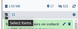
- Click on galaxy-selector Select Items at the top of the history panel
- Check all the datasets in your history you would like to include
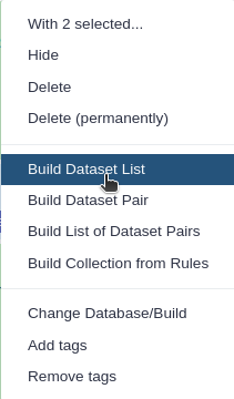
Click n of N selected and choose Advanced Build List
You are in collection building wizard. Choose Flat List and click ‘Next’ button at the right bottom corner.
Double clcik on the file names to edit. For example, remove file extensions or common prefix/suffixes to cleanup the names.
- Enter a name for your collection
- Click Build to build your collection
- Click on the checkmark icon at the top of your history again


Getting DAC access
Our test data is stored in EGA, which can be easily accessed using the EGA Download Client. Our specific EGA dataset accession ID is: “EGAD00001008392”. However, before you can access this data you need to request DAC access to this dataset. This can be requested by emailing to helpdesk@ega-archive.org, don’t forget to mention the dataset ID! When the EGA grants you access it will create an account for you, if you don’t have it already. Next, you should link your account to your Galaxy account by going to the homepage on Galaxy and at the top bar click User > Preferences > Manage Information. Now add your email and password of your (new) EGA account under: Your EGA (european Genome Archive) account. After that you can check if you can log in and see if you have access to the dataset.
Hands On: Check log-in and authorized datasets
- EGA Download Client ( Galaxy version 5.0.2+galaxy0) with the following parameters:
- “What would you like to do?”:
List my authorized datasetsComment: Check if the dataset is listed.Check if your dataset is listed in the output of the tool. If not you can look at the header of the output to find out why it is not listed. When the header does not provide any information you could have a look at the error message by clicking on the eye galaxy-eye of the output dataset and then click on the icon view details details. The error should be listed at Tool Standard Error.
Download list of files
When you have access to the EGA dataset, you can download all the needed files. However, the EGA dataset contains many different filetypes and cases, but we are only interested in the VCFs from case 5 and, to reduce execution time, the variants on chromosome 17. To be able to donwload these files we first need to request the list of files from which we can download. Make sure to use version 4+ of the EGA Download Client ( Galaxy version 5.0.2+galaxy0).
Hands On: Request list of files in the dataset
- EGA Download Client ( Galaxy version 5.0.2+galaxy0) version 4+ with the following parameters:
- “What would you like to do?”:
List files in a datasets- “EGA Dataset Accession ID?”:
EGAD00001008392Tools are frequently updated to new versions. Your Galaxy may have multiple versions of the same tool available. By default, you will be shown the latest version of the tool.
Switching to a different version of a tool:
- Open the tool
- Click on the tool-versions versions logo at the top right
- Select the desired version from the dropdown list
Filter list of files
Now that we have listed all the files, we need to filter out the files we actually need. We can do this by using a simple regular expression or regex. With regex it will be easy to find or replace patterns within a textfile.
Hands On: Filter out VCFs from list of files
- Search in textfiles ( Galaxy version 1.1.1) with the following parameters:
- param-file “Select lines from”:
List of EGA datasets(output of EGA Download Client tool)- “Type of regex”:
Extended (egrep)- “Regular Expression”:
Case5.+17.+vcf.gz$The regex might seem a bit complicated if you never worked with it, however it is quite simple. We simply search for lines which contain our sequence of characters, which are lines that contain Case5 then any character for any length, denoted by the “.+”, until (chromosome) 17 is found and then again any character for any length until the sequence ends with, denoted by the dollar sign, “vcf.gz”.- “Match type”:
case sensitive
Download files
After the filtering you should have a tabular file with 3 lines each containing the ID of a VCF file from case 5, as shown below.
EGAF00005573839	1	33859685	53277d993a780e0c295079bf1346ee9f	Case5_IC.17.g.vcf.gz
EGAF00005573866	1	33350163	7e612852ee0824be458fbf9aeecaa61a	Case5_M.17.g.vcf.gz
EGAF00005573882	1	42856357	14b53924d1492e28ad6078ceb8cfdbc7	Case5_F.17.g.vcf.gz
Hands On: Download listed VCFs
- EGA Download Client ( Galaxy version 5.0.2+galaxy0) with the following parameters:
- “What would you like to do?”:
Download multiple files (based on a file with IDs)
- param-file “Table with IDs to download”:
Filtered list of files(output of Search in textfiles tool)- “Column containing the file IDs”:
Column: 1After the download you should have a collection with one file for each family member, i.e. mother (M), father (F), and case (IC). Make sure the files are recognized as the vcf_bgzip format.
- Click on the galaxy-pencil pencil icon for the dataset to edit its attributes
- In the central panel, click galaxy-chart-select-data Datatypes tab on the top
- In the galaxy-chart-select-data Assign Datatype, select
datatypesfrom “New Type” dropdown
- Tip: you can start typing the datatype into the field to filter the dropdown menu
- Click the Save button
Decompress VCFs
Finally, we need to decompress our bgzipped VCFs, since we will use a text manipulation tool as a next step to process the VCFs. To decompress the vcf we will use a built-in tool from Galaxy, which can be accessed by manipulating the file itself in a similair fashion as changing its detected type.
Hands On: Convert compressed vcf to uncompressed.Open the collection of VCFs and execute the following steps for each VCF.
Click on the pencil galaxy-pencil of the vcf you want to convert.
Click on the convert tab galaxy-gear.
Under Target datatype select
vcf (using 'Convert compressed file to uncompressed.')Click exchange Create Dataset.
After transforming all the VCFs you need to combine the converted VCFs into a colllection again.
- Click on galaxy-selector Select Items at the top of the history panel
- Check the 3 vcf files
Click 3 of N selected and choose Advanced Build List
You are in collection building wizard. Choose Flat List and click ‘Next’ button at the right bottom corner.
Double clcik on the file names to edit. For example, remove file extensions or common prefix/suffixes to cleanup the names.
- Enter a name for your collection
- Click Build to build your collection
- Click on the checkmark icon at the top of your history again
Pre-Processing
Before starting the analysis, the VCF files have to be pre-processed in order to meet input requirements of the tools which we will use for the downstream analysis.
Add chromosome prefix to vcf
Firstly, our next tool has some assumptions about our input VCFs. The tool expects the chromosome numbers to start with a prefix chr. Our VCFs only use the chromosome numbers however, the VCFs just use the chromosome numbers. This is due to a difference in reference genome used when creating the VCFs. To change the prefix in the VCFs we will use regex again.
Hands On: Add chr prefix using regex
- Column Regex Find And Replace ( Galaxy version 1.0.1) with the following parameters:
- param-file “Select cells from”:
VCFs(output of Convert compressed file to uncompressed. tool)- “using column”:
Column: 1- In “Check”:
- param-repeat “Insert Check”
- “Find Regex”:
^([0-9MYX])- “Replacement”:
chr\1- param-repeat “Insert Check”
- “Find Regex”:
^(##contig=<.*ID=)([0-9MYX].+)- “Replacement”:
\1chr\2Comment: Explaining the regex.The two regex patterns might look complicated but they are quite simple if you break them down in components.
- The first check
^([0-9MYX])>chr\1adds thechrprefix to all the non-header line. The check can be broken down into the following elements:
^means that the pattern has to start at the beginning of the line not somewhere randomly in the line.[0-9MYX]means that at this position there should be a character from the list[], namely either a number from0-9or the characterM,Y, orX.- The replacement pattern
chr\1means that the prefixchrhas to be inserted before the first match\1. Here the first match refers to the pattern in the first brackets()around the list[0-9MXY].- The second check
(##contig=<.*ID=)([0-9MYX].+)>\1chr\2adds thechrprefix to the contig ids in the header lines. The check can be broken down into the following elements:
- The first match, the pattern in the first brackets
##contig=<.*ID=, matches the contig header lines, which start with##contig=<. It is followed by a match anything.for zero-or-more times*until it findsID=.- The second match, the pattern in the second brackets
[0-9MYX].+, matches the chromosome numbers and characters[0-9MYX]followed by a matching anything.for one-or-more times+.- The replacement pattern
\1chr\2means that the prefixchrhas to be inserted between the first match\1or##contig=<.*ID=and the second match\2or[0-9MYX].+.
Normalizing VCF
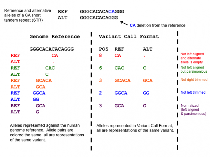
After adding the prefixes to the VCFs we need to normalize the variants in the VCF to standardize how the variants are represented within the VCF. This is a very important step, since the variants in the mother and daughter might be represented differently, which would mean that the causative variant might be overlooked!
One of the normalization steps is splitting multiallelic variants, 2 variants detected on the same position but on a different allele. Splitting these records will put the 2 variants on a separate line, that way the impact of the individual mutations can be evaluated. In addition, indels need to be left-aligned and normalized because that’s how they are stored in the annotation databases. An indel is left-aligned and normalized, according to Tan et al. 2015, “if and only if it is no longer possible to shift its position to the left while keeping the length of all its alleles constant” and “if it is represented in as few nucleotides as possible”.
 Open image in new tab
Hands On: Normalize VCF
- bcftools norm ( Galaxy version 1.9+galaxy1) with the following parameters:
- param-file “VCF/BCF Data”:
VCFs with chr prefix(output of Text reformatting tool)- “Choose the source for the reference genome”:
Use a built-in genome
- “Reference genome”:
Human (Homo sapiens): hg19- “Left-align and normalize indels?”:
Yes- “~multiallelics”:
split multiallelic sites into biallelic records (-)- In “Restrict all operations to”:
- “Regions”:
Do not restrict to Regions- “Targets”:
Do not restrict to Targets- “output_type”:
uncompressed VCFYou can have a look at the summary to check what changes were made. First, expand the output of bcftools norm (by clicking on the box) and it should be listed in the box. If not you can find it by clicking on the icon view details details and look at the output of the ToolStandard Error.
Filter NON_REF sites
After normalizing the VCFs we will filter out the variants with a NON_REF tag in the ALT column, the column which represents the mutated nucleotide(s). According to the header, these sites correspond to: “any possible alternative allele at this location”. So these sites are a sort of placeholders for potential variants. However we are not interested in this kind of variants and they slow our analysis down quite a lot, so we will filter them out.
Hands On: Filter out NON_REF sites
- Filter with the following parameters:
- param-file “Filter”:
Normalized VCFs(output of bcftools norm tool)- “With following condition”:
c5!='<NON_REF>'- “Number of header lines to skip”:
142This has to be set manually since the tool skips lines starting with ‘#’ automatically.
Question
- Why didn’t we filter out the NON_REF site directly after filtering? Have a look at the VCFs before and after normalization.
- Could we have filtered out the NON_REF sites earlier with a different program?
- The
<NON_REF>sites were sometimes also represented as a multi allelic variant e.g.,chr17 302 . T TA,<NON_REF>which would not be filtered out with the Filter tool.- Possibly, if the
<NON_REF>variants were filtered out and if the<NON_REF>tag was removed from multi-allelic variants. However, the last task (splitting multi-allelic sites) can already be handled by bcftools norm ( Galaxy version 1.9+galaxy1) and it might involve more sophisticated steps to properly split these variants.
Merge VCF collection into one dataset
Finally, we can merge the 3 separate files of the parents and patient into a single VCF. This will put overlapping variants on the same line by aligning the samples format column. If a sample misses a certain variant then on the line of that variant the sample’s format information will look like this: ./.:.:.:.:.:.. This makes it easier to find shared and missing variants between the parents and ofspring. A tool which can do this is the bcftools merge ( Galaxy version 1.10) tool.
Hands On: Merge VCFs
- bcftools merge ( Galaxy version 1.10) with the following parameters:
- param-file “Other VCF/BCF Datasets”:
<NON_REF> filtered VCFs(output of Text reformatting tool)- In “Restrict to”:
- “Regions”:
Do not restrict to Regions- In “Merge Options”:
- “Merge”:
none - no new multiallelics, output multiple records instead- “output_type”:
uncompressed VCFComment: Checking the merged VCF.Check the merged VCF, now each line should contain 3 sample columns, namely
Case6F,Case6M, andCase6C. These columns represent the presence of the variant for the mother, father, and offspring.
Annotation
To understand what the effect of our variants are, we need to annotate our variants. We will use the tool SnpEff eff ( Galaxy version 4.3+T.galaxy1), which will compare our variants to a database of variants with known effects.
Annotate with SNPeff
Running SnpEff will produce the annotated VCF and an HTML summary file. The annotations are added to the INFO column in the VCF and the added INFO IDs (ANN, LOF, and NMD) are explained in the header. The summary files include the HTML stats file which contains general metrics, such as the number of annotated variants, the impact of all the variants, and much more.
Hands On: Annotation with SnpEff
- SnpEff eff: ( Galaxy version 4.3+T.galaxy1) with the following parameters:
- param-file “Sequence changes (SNPs, MNPs, InDels)”:
Merged VCF(output of bcftools merge tool)- “Output format”:
VCF (only if input is VCF)- “Genome source”:
Locally installed snpEff database
- “Genome”:
Homo sapiens : hg19- “spliceRegion Settings”:
Use Defaults- “Filter out specific Effects”:
No
Question
- How many variants got annotated?
- Is there something notable you can see from the HTML file?
- The number of variants processed is 209,143.
- Most variants are found in the intronic regions. However, this is to be expected since the mutations in intonic regions generally do not affect the gene.
Compress VCF
Now that we have finished running all the tools which require the VCF format as input, they can be converted back to the vcf_bgzip format. To compress the VCF we will use a built-in tool from Galaxy, which can be accessed by manipulating the file itself in a similair fashion as changing its detected type.
Hands On: Compress **vcf** back to **vcf_bgzip**Execute the following steps for the SnpEff VCF.
Click on the pencil galaxy-pencil of the SnpEff VCF.
Click on the convert tab galaxy-gear.
Under Target datatype select
vcf_bgzip (using 'Convert uncompressed file to compressed.')Click exchange Create Dataset.
Trio Analysis
GEMINI analyses
Next, we will transform our VCF into a GEMINI database which makes it easier to query the VCFs and to determine different inheritence patterns between the mother, father, and offspring. In addition, GEMINI will add even more annotations to the variants. This allows us to filter the variants even more which gets us to closer to the real causative variant. All these steps are performed by the GEMINI load ( Galaxy version 0.20.1+galaxy2) tool. However, before we can load the VCF we also need to define a pedigree file.
Create a pedigree file describing the family trio
A pedigree file is a file that informs GEMINI which family members are affected by the disease and which sample name corresponds to what individual. This information is saved as a table containing information about the phenotype of the family.
- #family_id: Which family a row belongs to.
- name: The name of the sample, note this sample name has to overlap with the sample name in the VCF, see the last 3 columns of the VCF. However, for some reason the VCF contains the sample name from case 6 and not case 5. This was probably just a typo in the VCF, however here we just copy the sample name to our pedigree file.
- paternal_id: The sample name of the father or 0 for missing.
- maternal_id: The sample name of the mother or 0 for missing.
- sex: The sex of the person.
- phenotype: Wether or not the person is affected by the disease.
Hands On: Creating the PED file
- Upload the pedigree file from below.
#family_id	name	paternal_id	maternal_id	sex	phenotype
FAM0001822	Case6M	0	0	2	2
FAM0001822	Case6F	0	0	1	1
FAM0001822	Case6C	Case6F	Case6M	2	2
- Click galaxy-upload Upload Data at the top of the tool panel
- Select galaxy-wf-edit Paste/Fetch Data at the bottom
- Paste the file contents into the text field
- Press Start and Close the window
For more information on the PED file you can read the help section of the GEMINI load ( Galaxy version 0.20.1+galaxy2) tool in the description, which can be found at the bottom of the page when clicking on the tool.
Load GEMINI database
Now we can transform the subsampled VCF and PED file into a GEMINI database. Note that this can take a very long time depending on the size of the VCF. In our case it should take around 30-40 minutes.
Hands On: Transform VCF and PED files into a GEMINI database
- GEMINI load ( Galaxy version 0.20.1+galaxy2) with the following parameters:
- param-file “VCF dataset to be loaded in the GEMINI database”:
SnpEff Annotated vcf_bgzip(output of Convert uncompressed file to compressed. tool)- param-file “Sample and family information in PED format”: the pedigree file prepared above
Find inheritance pattern
With the GEMINI database it is now possible to identify the causative variant that could explain the breast cancer in the mother and daughter. The inheritance information makes it a bit easier to determine which tool to run to find the causative variant, instead of finding it by trying all the different inheritance patterns.
QuestionWhich inheritance pattern could have occurred in this family trio?
The available inheritance patterns can be found in the GEMINI inheritance pattern ( Galaxy version 0.20.1) tool.
- Since both the daughter and mother are affected, and the father likely unaffected1, the mutation is most probably dominant. The disease could still be recessive if the father has one copy of the faulty gene, however this is less likely.
- The mutation is most likely not de-novo, since both the daughter and mother are affected.
- The mutation could be X-linked, however since the VCF only contain mutations on chromosome 17 it would practically be impossible.
- The disease could be compound heterozygous, however in that case the disease should be recessive which is less likely.
- A loss of heterozygosity (LOH) is also possible, since it is a common occurrence in cancer so this could be a viable inheritance pattern.
Based on these findings it would make sense to start looking for inherited autosomal dominant variants as a first step. If there are no convincing candidate mutations it would always be possible to look at the other less likely inheritance patterns, namely de-novo, compound heterozygous, and LOH events.
To find the most plausible causative variant we will use the GEMINI inheritance pattern ( Galaxy version 0.20.1) tool. This tool allows us to select the most likely inheritance pattern (autosomal dominant). Below it is explained how to run the tool for this specific pattern, but you can always try other inheritence patterns if you are curious.
Hands On: Run GEMINI autosomal dominant inhertiance pattern
- GEMINI inheritance pattern ( Galaxy version 0.20.1) with the following parameters:
- param-file “GEMINI database”:
GEMINI database(output of GEMINI load tool)- “Your assumption about the inheritance pattern of the phenotype of interest”:
Autosomal dominant
- In “Additional constraints on variants”:
- param-repeat “Insert Additional constraints on variants”
- “Additional constraints expressed in SQL syntax”:
impact_severity != 'LOW'To filter variants on their functional genomic impact we will use the impact_severity feature. Here a low severity means a variant with no impact on protein function, such as silent mutations.- In “Family-wise criteria for variant selection”:
- “Specify additional criteria to exclude families on a per-variant basis”:
No, analyze all variants from all included families- In “Output - included information”:
- “Set of columns to include in the variant report table”:
Custom (report user-specified columns)
- “Additional columns (comma-separated)”:
chrom, start, ref, alt, impact, gene, clinvar_sig, clinvar_disease_name, clinvar_gene_phenotype, rs_ids
QuestionDid you find the causative variant in the output of the GEMINI inheritance pattern tool?
The only pathogenic variant related to breast cancer in the output, according to clinvar, is a SNP at chr17 at position 41215919 on the BRCA1 gene which transforms a G into a T, which is shown below.
chr17 41215919 G T missense_variant BRCA1 pathogenic,otherThis missense mutation transforms an alanine amino acid into a glutamine amino acid. Even though this variant has an unknown clinical significance in BRCA1 it was found to be among the top 10 SNPs which likely leads to breast cancer, according to Easton et al. 2007. You can find more info on this mutation by googling it’s rs_ID rs28897696.
Gene.iobio Analyses
Alternatively, the trio analysis can be done using gene.iobio Sera et al. 2021. The gene.iobio visualisation ( Galaxy version 4.7.1) tool generates an html file which sends the VCFs to the iobio site using public URLs. Therefore, your history has to be shared, i.e. everyone with a link can access your history!
Hands On: Make files accessible for gene.iobio
- Open the History Options menu galaxy-dropdown at the topright corner of your history panel.
- select Share or Publish workflow.
- Then toggle the galaxy-toggle Make History accessible.
For this tool it is not required to set any filtering steps or determine the most plausible inheritence pattern. Since gene.iobio runs multiple default filtering steps for autosomal dominant, recessive, De novo, compound heterozygous, and X-linked recessive inheritance patterns. In addition, it prioritizes variants based on gene-disease association algorithms, which significantly reduces processing time.
Hands On: Generate gene.iobio html
- gene.iobio visualisation ( Galaxy version 4.7.1) with the following parameters:
- param-file “Proband VCF file”:
SnpEff Annotated vcf_bgzip(output of Convert compressed file to uncompressed. tool)- “Proband sex”:
Female- “Proband sample name”:
Case6C- “Single/Trio analysis”:
Trio
- In “Father input”:
- param-file “Father VCF file”:
SnpEff Annotated vcf_bgzip(output of Convert compressed file to uncompressed. tool)- “Father sample name”:
Case6F- In “Mother input”:
- param-file “Mother VCF file”:
SnpEff Annotated vcf_bgzip(output of Convert compressed file to uncompressed. tool)- “Is the mother affected?”:
Yes- “Mother sample name”:
Case6M- “Select reference genome version”:
GRCh37To open the generated html file click on the eye galaxy-eye, which will show the gene.iobio interface. Now a phenotype has to be added to generate a list of genes which likely contain causative variants, in this case it is breast cancer. Next, click on the Hamburger icon in the topleft corner of the gene.iobio interface. This will show 20 genes including the BRCA1 gene with the causative variant under the Genes tab. Click on the BRCA1 gene and gene.iobio starts analyzing the gene for causative variants. Then under the Variants tab you will find the causative variant listed. You can click on the variant block to see more information on it. A report will show with information on the type, location, and quality of the variant, the associated phenotype, the pathogenicity, the population frequency, conservation of the location of the variant, and the inheritence pattern (Autosomal dominant).
More genes can be analyzed in three ways 1) the generated list of genes associated with a phenotypm can be increased. 2) The list of genes associated with another phenotype can be combined with the current list of genes. 3) A gene can manually be added.
- To increase the number of genes in the generated list of genes click on the gear icon galaxy-gear in gene.iobio and click on the drop down box under Keep top n genes from phenotype search.
- To add more genes to the analysis type and select another phenotype in the top bar. After finding your phenotype of interest press enter and click Combine genes with current list in the pop-up screen.
- To add a single gene to the analysis type and select a gene name in the top bar. After finding your gene of interest press enter.
Conclusion
In this tutorial we have illustrated how to easily download a dataset of interest savely and securely from the EGA using the HTSGET protocol. In addition, we performed a trio analysis to find the causative variant in an autosomal dominant inherited disease. We pre-processed and annotated our VCFs using the SnpEff and found the causative variant using both the GEMINI and gene.iobio tool. With this workflow you can now easily analyse and find the causative variant(s) in many different family trios from any database which HTSGET can connect to.
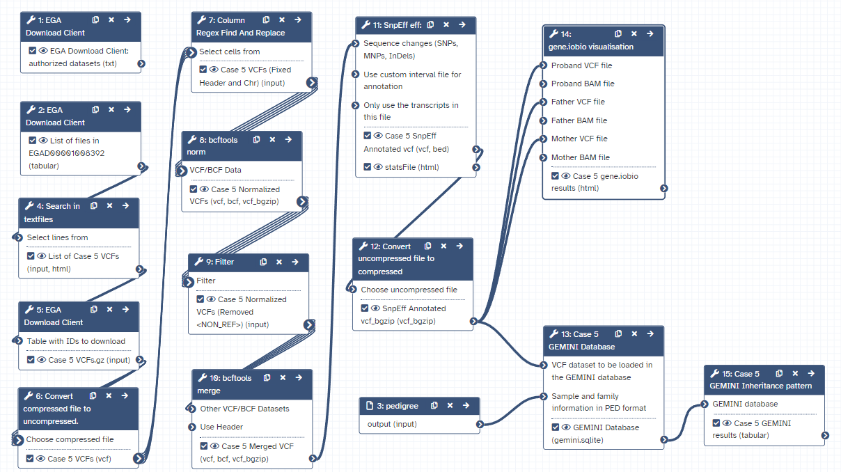
Workflow
Here is the final layout of the workflow. For more details you can download the workflow from the overview at the top of the page.
 Open image in new tab
-
It is unlikely that the father has breast cancer, “For men, the lifetime risk of getting breast cancer is about 1 in 833” via cancer.org ↩
You've Finished the Tutorial
Key points
Downloading whole datasets with HTSGET is safe and easy with Galaxy.
Regex is a usefull tool for pre-processing VCF files.
Variant annotations allows us to strictly filter VCFs to find the causative variant.
Frequently Asked Questions
Have questions about this tutorial? Have a look at the available FAQ pages and support channelsUseful literature
Further information, including links to documentation and original publications, regarding the tools, analysis techniques and the interpretation of results described in this tutorial can be found here.
References
- Easton, D. F., A. M. Deffenbaugh, D. Pruss, C. Frye, R. J. Wenstrup et al., 2007 A Systematic Genetic Assessment of 1, 433 Sequence Variants of Unknown Clinical Significance in the BRCA1 and BRCA2 Breast Cancer–Predisposition Genes. The American Journal of Human Genetics 81: 873–883. 10.1086/521032
- Tan, A., G. R. Abecasis, and H. M. Kang, 2015 Unified representation of genetic variants. Bioinformatics 31: 2202–2204. 10.1093/bioinformatics/btv112
- Eberle, M. A., E. Fritzilas, P. Krusche, M. Källberg, B. L. Moore et al., 2017 A reference data set of 5.4 million phased human variants validated by genetic inheritance from sequencing a three-generation 17-member pedigree. Genome Res. 27: 157–164. 10.1101/gr.210500.116
- Sera, T. D., M. Velinder, A. Ward, Y. Qiao, S. Georges et al., 2021 Gene.iobio: an interactive web tool for versatile, clinically-driven variant interrogation and prioritization. Scientific Reports 11: 10.1038/s41598-022-09959-3
Feedback
Did you use this material as an instructor? Feel free to give us feedback on how it went.
Did you use this material as a learner or student? Click the form below to leave feedback.

Citing this Tutorial
- Jasper Ouwerkerk, Wolfgang Maier, Helena Rasche, Saskia Hiltemann, Trio Analysis using Synthetic Datasets from RD-Connect GPAP (Galaxy Training Materials). https://training.galaxyproject.org/training-material/topics/variant-analysis/tutorials/trio-analysis/tutorial.html Online; accessed TODAY
- Hiltemann, Saskia, Rasche, Helena et al., 2023 Galaxy Training: A Powerful Framework for Teaching! PLOS Computational Biology 10.1371/journal.pcbi.1010752
- Batut et al., 2018 Community-Driven Data Analysis Training for Biology Cell Systems 10.1016/j.cels.2018.05.012
Congratulations on successfully completing this tutorial!@misc{variant-analysis-trio-analysis, author = "Jasper Ouwerkerk and Wolfgang Maier and Helena Rasche and Saskia Hiltemann", title = "Trio Analysis using Synthetic Datasets from RD-Connect GPAP (Galaxy Training Materials)", year = "", month = "", day = "", url = "\url{https://training.galaxyproject.org/training-material/topics/variant-analysis/tutorials/trio-analysis/tutorial.html}", note = "[Online; accessed TODAY]" } @article{Hiltemann_2023, doi = {10.1371/journal.pcbi.1010752}, url = {https://doi.org/10.1371%2Fjournal.pcbi.1010752}, year = 2023, month = {jan}, publisher = {Public Library of Science ({PLoS})}, volume = {19}, number = {1}, pages = {e1010752}, author = {Saskia Hiltemann and Helena Rasche and Simon Gladman and Hans-Rudolf Hotz and Delphine Larivi{\`{e}}re and Daniel Blankenberg and Pratik D. Jagtap and Thomas Wollmann and Anthony Bretaudeau and Nadia Gou{\'{e}} and Timothy J. Griffin and Coline Royaux and Yvan Le Bras and Subina Mehta and Anna Syme and Frederik Coppens and Bert Droesbeke and Nicola Soranzo and Wendi Bacon and Fotis Psomopoulos and Crist{\'{o}}bal Gallardo-Alba and John Davis and Melanie Christine Föll and Matthias Fahrner and Maria A. Doyle and Beatriz Serrano-Solano and Anne Claire Fouilloux and Peter van Heusden and Wolfgang Maier and Dave Clements and Florian Heyl and Björn Grüning and B{\'{e}}r{\'{e}}nice Batut and}, editor = {Francis Ouellette}, title = {Galaxy Training: A powerful framework for teaching!}, journal = {PLoS Comput Biol} }
You can use Ephemeris's
shed-tools installcommand to install the tools used in this tutorial.shed-tools install [-g GALAXY] [-a API_KEY] -t <(curl https://training.galaxyproject.org/training-material/api/topics/variant-analysis/tutorials/trio-analysis/tutorial.json | jq .admin_install_yaml -r)Alternatively you can copy and paste the following YAML
---
install_tool_dependencies: true
install_repository_dependencies: true
install_resolver_dependencies: true
tools:
- name: text_processing
  owner: bgruening
  revisions: d698c222f354
  tool_panel_section_label: Text Manipulation
  tool_shed_url: https://toolshed.g2.bx.psu.edu/
- name: regex_find_replace
  owner: galaxyp
  revisions: ae8c4b2488e7
  tool_panel_section_label: Text Manipulation
  tool_shed_url: https://toolshed.g2.bx.psu.edu/
- name: bcftools_merge
  owner: iuc
  revisions: 86296490704e
  tool_panel_section_label: Variant Calling
  tool_shed_url: https://toolshed.g2.bx.psu.edu/
- name: bcftools_norm
  owner: iuc
  revisions: da6fc9f4a367
  tool_panel_section_label: Variant Calling
  tool_shed_url: https://toolshed.g2.bx.psu.edu/
- name: ega_download_client
  owner: iuc
  revisions: 7d87a9d58aa1
  tool_panel_section_label: Get Data
  tool_shed_url: https://toolshed.g2.bx.psu.edu/
- name: gemini_inheritance
  owner: iuc
  revisions: 2c68e29c3527
  tool_panel_section_label: Gemini
  tool_shed_url: https://toolshed.g2.bx.psu.edu/
- name: gemini_load
  owner: iuc
  revisions: 2270a8b83c12
  tool_panel_section_label: Gemini
  tool_shed_url: https://toolshed.g2.bx.psu.edu/
- name: geneiobio
  owner: iuc
  revisions: c0af7b196a89
  tool_panel_section_label: Graph/Display Data
  tool_shed_url: https://toolshed.g2.bx.psu.edu/
- name: snpeff
  owner: iuc
  revisions: 5c7b70713fb5
  tool_panel_section_label: Variant Calling
  tool_shed_url: https://toolshed.g2.bx.psu.edu/