AskOmics is a web application for data integration and querying using the Semantic Web technologies. It helps users to convert multiple data sources (CSV/TSV files, GFF and BED annotation) into “RDF triples” and store them in a specific kind of database: an “RDF triplestore”. Under this form, data can then be queried using a specific language: “SPARQL”. AskOmics hides the complexity of these technologies and allows to perform complex queries using a user-friendly interface.
AskOmics comes in useful for cross-referencing results datasets with various reference data. For example, in RNA-Seq studies, we often need to filter the results on the fold change and the p-value, to get the most significant differentially expressed genes. If you are studying a particular phenotype and already know the position of some QTL associated to this phenotype, you would then want to find the positions of the differentially expressed genes and determine which gene is located within one of those QTL. Finally, you would want to know if these genes have human homologs, and use the neXtProt database to get the location of the proteins coded by the homologs. The whole process involves several tools to parse and manipulate the different data format, and to map datasets on each other. AskOmics offer a solution to 1) automatically convert the multiple formats to RDF, 2) use a user-friendly interface to perform complex SPARQL queries on the RDF datasets to find the genes you are interested in, and 3) connect external SPARQL databases and link external data with your own.
In this tutorial, we will use results from a differential expression analysis. This file is provided for you below. You could also generate the file yourself, by following the RNA-Seq counts to gene tutorial. The file used here was generated from limma-voom but you could use a file from any RNA-seq differential expression tool, such as edgeR or DESeq2, as long as it contains the required columns (see below).
The differentially expressed results will be linked to the official mouse genome annotation, in general feature format (GFF). The file provided is a subset of the mouse annotation (GRCm38.p6) obtained from Ensembl.
We will use a file containing quantitative trait loci (QTL) information, to find if our differentially expressed genes are located inside a known QTL. This file is a subset of a query performed on Mouse Genome Informatics.
A file containing all homologies between mouse and human will be used to get the human homolog genes. This file is provided by MGI.
In the differentially expressed file, and the homologs file, gene are described by a symbol (e.g. Pwgrq10). However, in the annotation file and neXtProt database, gene are represented by Ensembl id (e.g. ENSMUSG00000025969). To link the 2 datasets, we will need a file to map the gene symbol with Ensembl id. This file provided for you was previously generated with an AskOmics query on the mouse annotation file and the homolog file.
To link the human gene with neXtProt database, we will use the RDF abstraction of neXtProt. This file was obtained using the Abstractor tool.
During the integration step, AskOmics builds an RDF description of the data: the abstraction. This abstraction is used to explore the data and build the query.
AskOmics can also integrate abstraction of distant endpoint. Abstraction are obtained using abstractor, a python package to generate RDF abstractions from distant endpoints.
The query builder interface is used to create a path through the abstraction of each ressources. The path is converted to a SPARQL query that is sent to the multiple SPARQL endpoint.
Differentially expressed results file (genes in rows, and 4 required columns: identifier (ENTREZID), gene symbol (SYMBOL), log fold change (logFC) and adjusted P values (adj.P.Val))
Reference genome annotation file (in GFF format)
QTL file (QTL in rows, with 5 required columns: identifier, chromosome, start, end and name)
Homolog file (TSV of 13 columns including homolog id, organism name and gene symbol)
Correspondence file between gene symbol and Ensembl id (TSV of 3 columns: symbol, the corresponding Ensembl id (mouse and human)
neXtProt abstraction (RDF data description of neXtProt database in turtle format)
Import data
Hands On: Data upload
Create a new history for this RNA-seq exercise e.g. RNA-seq AskOmics
To create a new history simply click the new-history icon at the top of the history panel:
Click on galaxy-pencil (Edit) next to the history name (which by default is “Unnamed history”)
Type the new name
Click on Save
To cancel renaming, click the galaxy-undo “Cancel” button
If you do not have the galaxy-pencil (Edit) next to the history name (which can be the case if you are using an older version of Galaxy) do the following:
Click on Unnamed history (or the current name of the history) (Click to rename history) at the top of your history panel
Type the new name
Press Enter
Import the files.
To import the files, there are two options:
Option 1: From a shared data library if available (ask your instructor)
Rename the files using the galaxy-pencil (pencil) icon.
limma-voom_luminalpregnant-luminallactate to DE results
Mus_musculus.GRCm38.98.subset.gff3 to Mus musculus annotation
Symbol.tsv to Gene Symbols
MGIBatchReport_Qtl_Subset.txt to QTL
HOM_MouseHumanSequence.rpt to Homolog groups
nextprot_asbtraction.ttl to neXtProt abstraction
Check every datatype.
DE results: tabular
Mus musculus annotation: gff
Gene Symbol: tabular
QTL: tabular
Homolog groups: tabular
neXtprot abstraction: ttl
If the datatypes are wrong, please change it.
Click on the galaxy-pencilpencil icon for the dataset to edit its attributes
In the central panel, click galaxy-chart-select-dataDatatypes tab on the top
In the galaxy-chart-select-dataAssign Datatype, select your desired datatype from “New Type” dropdown
Tip: you can start typing the datatype into the field to filter the dropdown menu
Click the Save button
Click on the galaxy-eye (eye) icon and take a look at the uploaded files.
Two step are necessary to get our data converted into RDF triples. The first step is to upload the Galaxy datasets into the AskOmics server. The second step is to integrate the uploaded data into the RDF triplestore.
Upload inputs into AskOmics
We will first launch an AskOmics interactive tool, and upload the data into it.
Launch AskOmics Interactive Tool
Hands On: Launch AskOmics IT
AskOmics a visual SPARQL query builder tool to launch the Interactive Tool
param-file“Datasets to load into AskOmics”: DE results, Mus musculus annotation, Gene Symbols, QTL, Homolog groups and neXtProt abstraction
Wait a few seconds (or minutes if computing resources are busy) for AskOmics to be ready to use. A view link should appear in the confirmation box just after clicking on the Execute button.
AskOmics is an Interactive tool. It means that when you launch it, it will stay in running state (yellow background) in your History. As long as it stays in this running state, you can access it by looking in the “User” > “Active Interactive Tools” menu (click on its name to view it). When you no longer need it, you can stop it by deleting it from your history, or using the “Stop” button in the “User” > “Active Interactive Tools” page.
Keep in mind that as long as this tool runs, it uses computing resources, so don’t forget to stop it when you no longer have use for it.
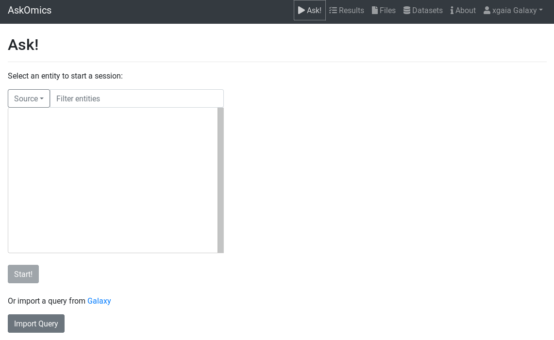
Once the AskOmics Interactive Tool is ready, you should see a start page looking like this:
The TSV preview shows an HTML table representing the first lines of the TSV file. During integration, AskOmics will convert the file using the header.
The first column of a TSV file will be the entity name. Other columns of the file will be attributes of the entity. Labels of the entity and attributes will be set by the header. Each label can be edited by clicking on it.
Entity and attributes can have special types. The types are defined with the select box below the header. An entity can be a start entity or an entity. A start entity means that the entity may be used to start a query on the AskOmics homepage.
Attributes can take the following types:
Numeric: if all the values of the column are numeric
Text: if all the values are strings
Category: if there is a limited number of repeated values (e.g. ‘green’, ‘yellow’ and ‘red’, each one found in multiple lines)
If the entity describes a locatable element on a genome:
Reference: chromosome
Strand: strand
Start: start position
End: end position
A column can also represent a relation between the entity to another. In this case, the header have to be named relationName@TargetedEntity and the type Directed or Symetric relation. A Directed relation is a relation from this entity to the targeted one (e.g. A is B’s father, but B is not A’s father). A Symetric relation is a relation that works in both directions (e.g. A loves B, and B loves A).
Hands On: Integrate `DE results`
Search for DE results (preview)
Edit attribute names and types:
change ENTREZ ID to Differential Expression and set type to start entity
change SYMBOL to linkedTo@Gene Symbol and set type to Symetric relation
change GENENAME to name and set type to text
Keep the other column names and set their types to numeric
The last dataset we want to integrate is the neXtProt abstraction. This file contains some RDF data that instructs AskOmics how to communicate with a remote RDF database containing neXtProt data.
Hands On: Integrate `neXtProt abstraction`
Search for neXtProt abstraction (preview)
Check that Distant endpoint is set to https://sparql.nextprot.org/sparql in advanced options
Once all the data of interest is integrated (converted to RDF), its time to query them. Querying RDF data is done by using the SPARQL language. Fortunately, AskOmics provides a user-friendly interface to build SPARQL queries without having to learn the SPARQL language.
Query builder overview
Simple query
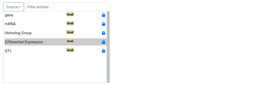
The first step to build a query is to choose a start point for the query.
Once the start entity is chosen, the query builder is displayed.
The query builder is composed of a graph. Nodes represents entities and links represents relations between entities. The selected entity is surrounded by a red circle. Links and other entities are dotted and lighter because there are not instantiated.
Figure 11: Query builder, Differential Expression is the selected entity, Gene Symbol is a suggested entity
On the right, attributes of the selected entity are displayed as attribute boxes. Each box has an eye icon: an opened eye means the attribute will be displayed on the results.
Hands On: Ask for all Differential Expression and display some attributes
Display logFC and adj.P.val by clicking on the eye icon
Run & preview launch the query with a limit of 30 rows returned. We use this button to get an idea of the results returned.
Filter on attributes
Next query will search for all over-expressed genes. Genes are considered over-expressed if the log fold change is > 2. We are only interested by significant results (Adj P value ≤ 0.05)
Back to the query builder,
Hands On: Filter attributes to get significant over-expressed genes
Results now show the Ensembl id of our over-expressed genes. We have now access to all the information about the gene entity contained in the GFF file. For example, we can filter on chromosome and display chromosome and strand to get information about gene location.
AskOmics is able to perform special queries between entities that are locatable. These queries are:
Entities overlapping another one
Entities included in another entity
The FALDO ontology describes sequence feature positions and regions. AskOmics uses FALDO ontology to represent entity positions. GFF are using FALDO, as well as TSV entities with chromosome, strand, start and end.
On the query builder interface, locatable entities are represented with a green circle and relations based on location are represented as green arrow.
Hands On: Filter `gene`
First, remove the reference filter (unselect X using ctrl+click)
Remove the strand filter (unselect + using ctrl+click)
Hide referencestrand using the eye
Instantiate QTL
Click on the link between gene and QTL to edit the relation
Check that the relation is geneincluded inQTLon the same reference with strict ticked
To go further, we can filter on QTL to refine the results.
Hands On: Filter `gene`
Go back to the QTL node
Show the Name attribute using the eye icon
Filter the name with a regexp with growth
Run & preview
From now, our query is “All Genes that are over-expressed (logFC > 2 and FDR ≤ 0.05) and located on a QTL that is related to growth”. We can save this results with the Run & save button.
Hands On: Save a result
Run & save
Use neXtProt distant data to refine results
neXtProt is a comprehensive human-centric discovery platform, offering its users a seamless integration of and navigation through protein-related data. It offer a SPARQL endpoint that can be interrogated with AskOmics.
Since we added the neXtProt abstraction into our AskOmics instance, we can link our data to neXtProt.
Hands On: Find human homolog genes
Go back to the gene node
instantiate Gene Symbol and hide his Label
Instantiate Homolog Group, hide his label and filter his Common Organism Name with human
From Homolog Group, instantiate another Gene Symbol and hide his Label
Finally, follow the to neXtProt Gene link and instantiate Gene (with a capital G)
Run & preview
The query we’ve just built asks for the human homologs of our over-expressed genes. We use the Gene Symbol to get information from the neXtProt database. AskOmics converts the query into small SPARQL subqueries and send them to the local database and to the remote neXtProt endpoint.
Now we are linked to the neXtProt database, we can obtain information about the proteins encoded by these genes, as well as their location in the cell.
Hands On: Get the protein and their location
Instantiate Entry
Instantiate Isoform and hide the Label
Many nodes are connected to Isoform. Use the Filter links field to filter nodes linked with a link named location
Instantiate the Subcellular Location node and hide Uri
Use the Filter node field to filter nodes with “location” in their name
Instantiate Uniprot subcellular Location CV (you can use the node filter to clear up the screen)
Run & preview
Finally, our query is “All genes that are over-expressed and located on a QTL that is related to growth, their human homologs and the location of the proteins coded by this genes”. We will save it to the results.
Hands On: Save a result
Run & save
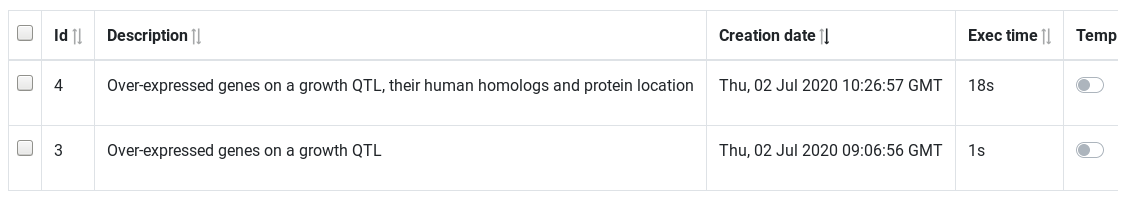
Results management
The results page displays the saved queries. Queries are sorted by creation date. At the end of the table, action buttons can be used to preview the result, download or send it to Galaxy history.
Hands On: Edit query name
Go to the Results page
Use the Preview button to check the result
Click on the name to rename the two query with Over-expressed genes on a growth QTL and Over-expressed genes on a growth QTL, their human homologs and protein location (press enter key to validate)
Now that you have used AskOmics to generate this final tabular file, you can continue analysing it with other Galaxy tools.
If you are done, don’t forget to close the AskOmics instance by going to the “User” > “Active Interactive Tools” page.
Conclusion
In this tutorial we have seen how to use AskOmics Interactive Tool. We launch the tools with a set of input files, then we have integrated these files into RDF and finally, we built complex queries over this local datasets and neXtProt to answer a biological question.
You've Finished the Tutorial
Please also consider filling out the Feedback Form as well!
Key points
AskOmics helps to integrate multiple data sources into an RDF database without prior knowledge in the Semantic Web
It can also be connected to external SPARQL endpoints, such as neXtProt
AskOmics helps to perform complex SPARQL queries without knowing SPARQL, using a user-friendly interface
Frequently Asked Questions
Have questions about this tutorial? Have a look at the available FAQ pages and support channels
Further information, including links to documentation and original publications, regarding the tools, analysis techniques and the interpretation of results described in this tutorial can be found here.
Feedback
Did you use this material as an instructor? Feel free to give us feedback on how it went.
Did you use this material as a learner or student? Click the form below to leave feedback.
Hiltemann, Saskia, Rasche, Helena et al., 2023 Galaxy Training: A Powerful Framework for Teaching! PLOS Computational Biology 10.1371/journal.pcbi.1010752
Batut et al., 2018 Community-Driven Data Analysis Training for Biology Cell Systems 10.1016/j.cels.2018.05.012
@misc{transcriptomics-rna-seq-analysis-with-askomics-it,
author = "Xavier Garnier and Anthony Bretaudeau and Anne Siegel and Olivier Dameron and Mateo Boudet",
	title = "RNA-Seq analysis with AskOmics Interactive Tool (Galaxy Training Materials)",
	year = "",
	month = "",
	day = "",
	url = "\url{https://training.galaxyproject.org/training-material/topics/transcriptomics/tutorials/rna-seq-analysis-with-askomics-it/tutorial.html}",
	note = "[Online; accessed TODAY]"
}
@article{Hiltemann_2023,
	doi = {10.1371/journal.pcbi.1010752},
	url = {https://doi.org/10.1371%2Fjournal.pcbi.1010752},
	year = 2023,
	month = {jan},
	publisher = {Public Library of Science ({PLoS})},
	volume = {19},
	number = {1},
	pages = {e1010752},
	author = {Saskia Hiltemann and Helena Rasche and Simon Gladman and Hans-Rudolf Hotz and Delphine Larivi{\`{e}}re and Daniel Blankenberg and Pratik D. Jagtap and Thomas Wollmann and Anthony Bretaudeau and Nadia Gou{\'{e}} and Timothy J. Griffin and Coline Royaux and Yvan Le Bras and Subina Mehta and Anna Syme and Frederik Coppens and Bert Droesbeke and Nicola Soranzo and Wendi Bacon and Fotis Psomopoulos and Crist{\'{o}}bal Gallardo-Alba and John Davis and Melanie Christine Föll and Matthias Fahrner and Maria A. Doyle and Beatriz Serrano-Solano and Anne Claire Fouilloux and Peter van Heusden and Wolfgang Maier and Dave Clements and Florian Heyl and Björn Grüning and B{\'{e}}r{\'{e}}nice Batut and},
	editor = {Francis Ouellette},
	title = {Galaxy Training: A powerful framework for teaching!},
	journal = {PLoS Comput Biol}
}
Congratulations on successfully completing this tutorial!
5 stars
1
July 2020
5 stars:
Liked: Very useful and well detailed presentation
Questions:


 Open image in new tab
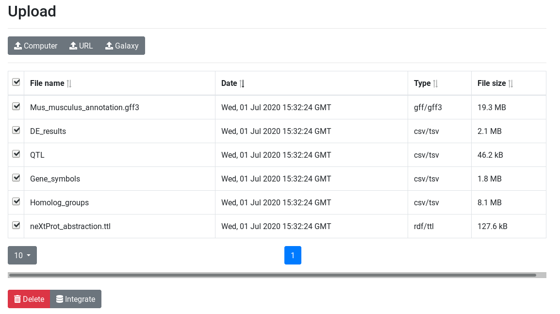 Open image in new tab
Open image in new tab
Open image in new tab
Open image in new tab
Open image in new tab
Open image in new tab
Open image in new tab
Open image in new tab
 Open image in new tab
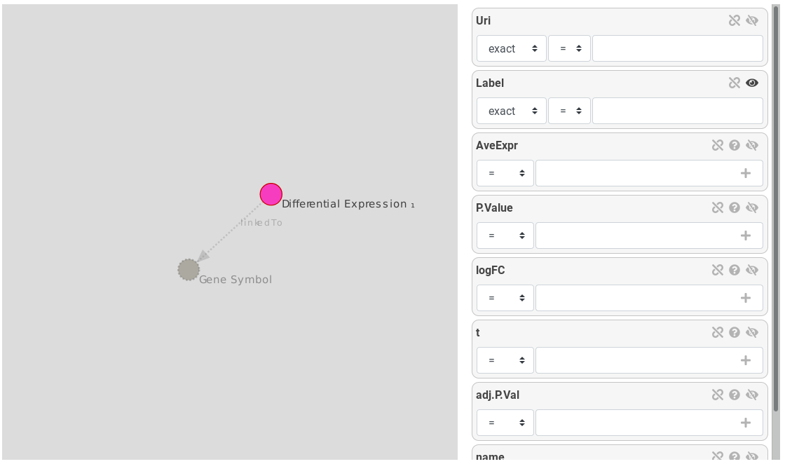 Open image in new tab
Open image in new tab
Open image in new tab
Open image in new tab
Open image in new tab
Open image in new tab
Open image in new tab
Open image in new tab
 Open image in new tab
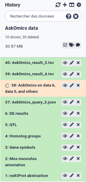 Open image in new tab