Statistical analysis of DIA data
| Author(s) |
|
| Reviewers |
|
OverviewQuestions:
Objectives:
How to perform statistical analysis on DIA mass spectrometry data?
How to detect and quantify differentially abundant proteins in a HEK-Ecoli Benchmark DIA datatset?
Requirements:
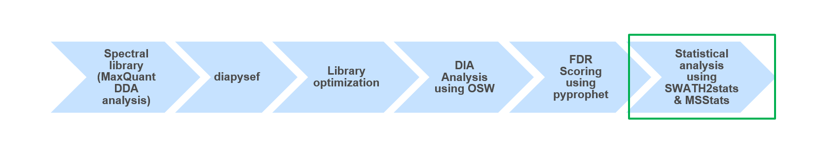
Statistical analysis of a HEK-Ecoli Benchmark DIA dataset
Understanding statistical approaches in proteomic analysis
Using MSstats to find significantly dysregulated proteins in a Spike-in dataset
- Introduction to Galaxy Analyses
- tutorial Hands-on: Library Generation for DIA Analysis
- tutorial Hands-on: DIA Analysis using OpenSwathWorkflow
Time estimation: 1 hourLevel: Intermediate IntermediateSupporting Materials:Published: Dec 2, 2020Last modification: Nov 9, 2023License: Tutorial Content is licensed under Creative Commons Attribution 4.0 International License. The GTN Framework is licensed under MITpurl PURL: https://gxy.io/GTN:T00210version Revision: 9
This training covers the statistical analysis of data independent acquisition (DIA) mass spectrometry (MS) data, after successfull identification and quantification of peptides and proteins. We therefore recommend to first go through the DIA library generation tutorial as well as the DIA analysis tutorial, which teach the principles and characteristics of DIA data analysis.
Modern mass spectrometry approaches enables the identification and quantification of thousands of proteins and tens of thousands of peptides in single measurements. This provides immense potential to in-depth explorative analysis of a variety of biological samples. However, often the number of available samples is limited leading to large proteomic datasets with only a few numbers of replicates or samples per condition. Thus, the statistical analysis remains challenging in such in-depth proteomic studies.
Here we will use MSstats, which enables the statistical analysis and processing of proteomic data (Choi et al. 2014).
AgendaIn this tutorial, we will cover:
Get data
Hands On: Data upload
Create a new history for this tutorial and give it a meaningful name
To create a new history simply click the new-history icon at the top of the history panel:
- Import the DIA analysis results, the sample annotation and the comparison matrix from Zenodo
https://zenodo.org/record/4307758/files/PyProphet_export.tabular
https://zenodo.org/record/4307758/files/Sample_annot_MSstats.txt
https://zenodo.org/record/4307758/files/Comp_matrix_HEK_Ecoli.txt
https://zenodo.org/record/4307758/files/PyProphet_msstats_input.tabular
- Copy the link location
Click galaxy-upload Upload at the top of the activity panel
- Select galaxy-wf-edit Paste/Fetch Data
Paste the link(s) into the text field
Press Start
- Close the window
Once the files are green, rename the sample annotation file in ‘Sample_annot_MSstats’, the comparison matrix file in ‘Comp_matrix_HEK_Ecoli’ and the two DIA analysis results files in ‘PyProphet_export’ and ‘PyProphet_msstats_input’
- Click on the galaxy-pencil pencil icon for the dataset to edit its attributes
- In the central panel, change the Name field
- Click the Save button


Statistical analysis with MSstats
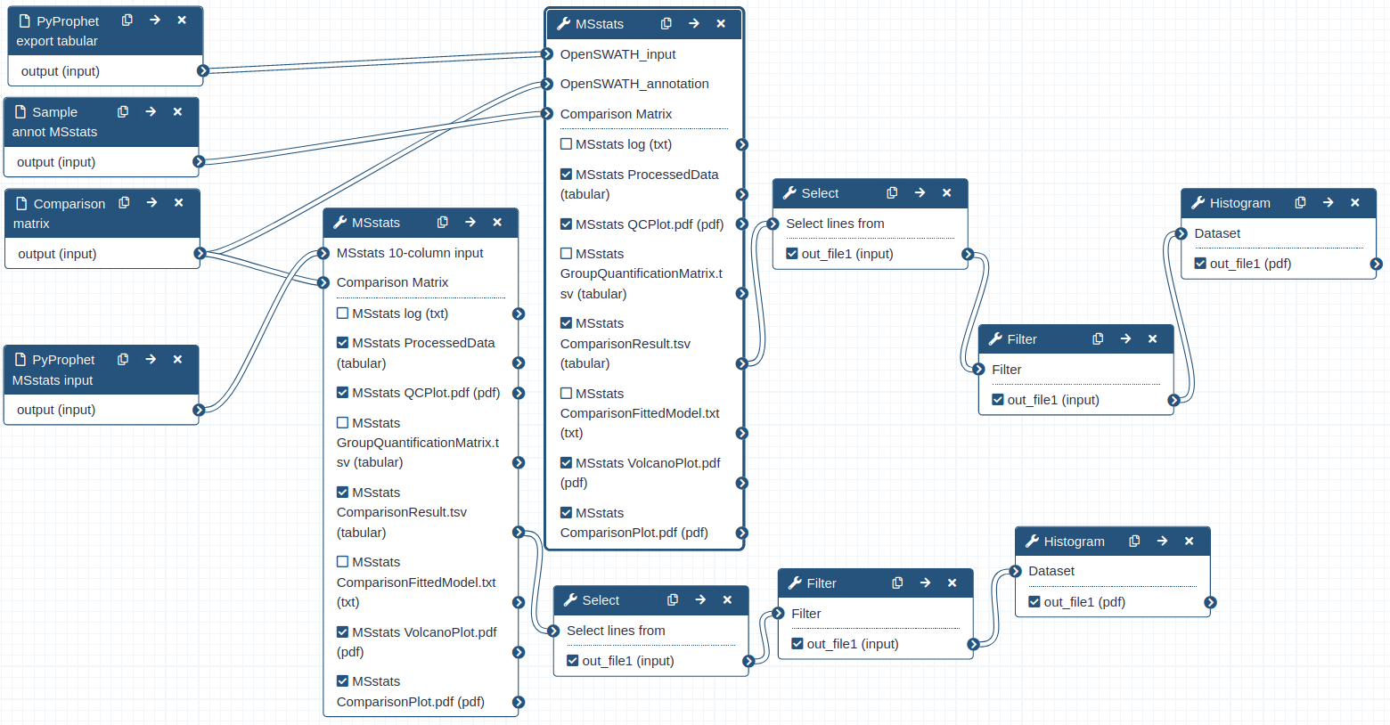
Hands On: Performing statistical analysis using MSstats and the tabular output from PyProphet export
- MSstats ( Galaxy version 3.20.1.0) with the following parameters:
- “input source”:
OpenSWATH
- param-file “OpenSWATH_input”:
PyProphet_export- param-file “OpenSWATH_annotation”:
Sample_annot_MSstats- “Compare Groups”:
Yes
- param-file “Comparison Matrix”:
Comp_matrix_HEK_EcoliComment: data Process and group comparisonDuring the data process step the peptide intensities are normalized and protein inference is performed. Using a predefined comparison matrix multiple comparisons can be performed.
Question
- How many lines does the PyPyprophet_export.tabular file have? How many lines does the ProcessedData have and do you notice any differences in their structure or format?
- How many proteins were used for the Group comparison? (see ComparisonResult)
- The PyPyprophet_export.tabular has appr. 230.000 lines whereas the ProcessedData has over 1 mio lines and is in the so called long format. Here every individual transition (single m/z value) is reported per row.
- The ComparisonResult has 5022 lines, meaning over 5000 Proteins were compared between the two different Spike-in conditions.
In case the MSstats run is not yet finished, the results can be downloaded from Zenodo to be able to continue the tutorial
- Import the files from Zenodo
https://zenodo.org/record/4307758/files/MSstats_ComparisonResult_export_tabular.tsv
Detailed investigation of Ecoli identifications and quantifications
Hands On: Investigating Ecoli proteins in the MSstats comparison results
- Select with the following parameters:
- param-file “Select lines from”:
MSstats_ComparisonResult_export_tabular(output of MSstats tool)- “the pattern”:
(ECOLI)|(log2FC)- Filter with the following parameters:
- param-file “Filter”:
Select_Ecoli(output of Select tool)- “With following condition”:
c7!='NA'- “Number of header lines to skip”:
1- Histogram ( Galaxy version 1.0.4) with the following parameters:
- param-file “Dataset”:
Filter_Ecoli(output of the previous Filter tool)- “Numerical column for x axis”:
Column: 3- “Number of breaks (bars)”:
25- “Plot title”:
Distribution of Ecoli Protein log FC values- “Label for x axis”:
log2 Fold ChangeComment: Extracting Ecoli informationFirst we only select rows containing specific terms such as “Ecoli” from the complete ComparisonResults file. Afterwards, the table is filtered to containg only proteins with valid statistical information (e.g. p-value). Using the log2 Fold change values from all remaining Ecoli proteins we can observe the distribution of log2FC values from the comparison of the two Spike-in conditions.
Question
- How many Ecoli proteins were identified and for how many was the p-value for the comparison of the two Spike-in conditions computed?
- How does the distribution of the log2FC values look like? Which Spike-in contained higher amounts of Ecoli and is it possible to see how much more Ecoli was spiked-in?
- In total, over 800 Ecoli proteins were identified from which 500 have a p-value for the comparison of the two Spike-in conditions.
- We can see a gaussian distribution of the log2FC values around a positive value of 3. Since we compared Spike_in_2 / Spike_in_1 we can directly see that Spike_in_2 contained higher amounts of Ecoli. Furthermore, since the apex of the distribution is around 3 and we compared log2 intensities, we could estimate that Spike_in_2 contained approx. 8-times more Ecoli than Spike_in_1.
Statistical analysis with MSstats
Hands On: Performing statistical analysis using MSstats and the msstats_input from PyProphet export
- MSstats ( Galaxy version 3.20.1.0) with the following parameters:
- “input source”:
MStats 10 column format
- param-file “MSstats 10-column input”:
PyProphet_msstats_input- “Compare Groups”:
YesComment: MSstats input formatFor the statistical analysis using MSstats the input must be in the long format, containing all relevant information in 10 predefined columns. The conversion of the PyProphet export output can either be done using MSstats (as we did above), or during the Pyprophet export step by using another R package called swath2stats (Blattmann et al. 2016). Prior to the conversion the data can be processed and filtered using the swath2stats functionalities.
Question
- How many lines does the
PyProphet_msstats_input.tabularfile have? How many lines does the ProcessedData have and do you notice any differences in their structure or format?- How many proteins were used for the Group comparison? And do you already see a difference to the first MSstats step?
- The
PyProphet_msstats_input.tabularhas over 870.000 lines and the ProcessedData has over 1 mio lines. Here both files are in the long format, in which every transition is reported per row.- Here the ComparisonResult has only 3871 lines, meaning that almonst 1200 fewer proteins were used in the comparison of the two spike-in conditions.
In case the MSstats run is not yet finished, the results can be downloaded from Zenodo to be able to continue the tutorial
- Import the files from Zenodo
https://zenodo.org/record/4307758/files/MSstats_ComparisonResult_msstats_input.tsv
Detailed investigation of Ecoli identifications and quantifications
Hands On: Investigating Ecoli proteins in the MSstats comparison results
- Select with the following parameters:
- param-file “Select lines from”:
MSstats_ComparisonResult_msstats_input(output of the second MSstats tool)- “the pattern”:
(ECOLI)|(log2FC)- Filter with the following parameters:
- param-file “Filter”:
Select_Ecoli(output of the second Select tool)- “With following condition”:
c7!='NA'- “Number of header lines to skip”:
1- Histogram ( Galaxy version 1.0.4) with the following parameters:
- param-file “Dataset”:
Filter_Ecoli(output of the previous Filter tool)- “Numerical column for x axis”:
Column: 3- “Number of breaks (bars)”:
25- “Plot title”:
Distribution of Ecoli Protein log FC values- “Label for x axis”:
log2 Fold Change
Question
- How many Ecoli proteins were identified and for how many was the p-value for the comparison of the two Spike-in conditions computed? Are there any differences compared to the selected and filtered results from the previous MSstats step?
- How does the distribution of the log2FC values look like? Are there any differences compared to the selected and filtered results from the previous MSstats step?
- In total, over 600 Ecoli proteins were identified from which 500 have a p-value for the comparison of the two Spike-in conditions. Here we identify 200 Ecoli proteins less than before, however, the number of proteins for which a p-value was calculated differs only slightly.
- Generally, the two log2FC distribution look very similar, showing a gaussian distribution of the log2FC values around a positive value of 3. There seems to be a slight difference of the apex of the distribution, in the first MSstats analysis it seems to be higher than 3, whereas in the second MSstats analysis the apex seems to be lower than 3.
Conclusion
 Open image in new tab
Using MSstats we were able to identify and quantify differentially regulated proteins between two Spike-in conditions in a HEK/Ecoli Benchmark DIA datatset. Furthermore, the preprocessing of the proteomic data prior to the statistical analysis can directly impact results. Thus, it might be beneficial to try various ways of intermediate data processing and statistical analysis to increase the sensitivity and specificity of the investigation.
 Open image in new tab
You've Finished the Tutorial
Key points
Statistical analyses are crucial for meaningful conclusion in proteomic studies
MSstats enables statistical analysis of data independent acquisition mass spectrometry data
Frequently Asked Questions
Have questions about this tutorial? Have a look at the available FAQ pages and support channelsUseful literature
Further information, including links to documentation and original publications, regarding the tools, analysis techniques and the interpretation of results described in this tutorial can be found here.
References
- Choi, M., C.-Y. Chang, T. Clough, D. Broudy, T. Killeen et al., 2014 MSstats: an R package for statistical analysis of quantitative mass spectrometry-based proteomic experiments. Bioinformatics 30: 2524–2526. 10.1093/bioinformatics/btu305 https://academic.oup.com/bioinformatics/bioinformatics/article/2748156/MSstats: ISBN: 1367-4811 (Electronic) 1367-4803 (Linking)
- Blattmann, P., M. Heusel, and R. Aebersold, 2016 SWATH2stats: An R/bioconductor package to process and convert quantitative SWATH-MS proteomics data for downstream analysis tools. PLoS ONE 11: 1–7. 10.1371/journal.pone.0153160
Feedback
Did you use this material as an instructor? Feel free to give us feedback on how it went.
Did you use this material as a learner or student? Click the form below to leave feedback.

Citing this Tutorial
- Matthias Fahrner, Melanie Föll, Statistical analysis of DIA data (Galaxy Training Materials). https://training.galaxyproject.org/training-material/topics/proteomics/tutorials/DIA_Analysis_MSstats/tutorial.html Online; accessed TODAY
- Hiltemann, Saskia, Rasche, Helena et al., 2023 Galaxy Training: A Powerful Framework for Teaching! PLOS Computational Biology 10.1371/journal.pcbi.1010752
- Batut et al., 2018 Community-Driven Data Analysis Training for Biology Cell Systems 10.1016/j.cels.2018.05.012
Congratulations on successfully completing this tutorial!@misc{proteomics-DIA_Analysis_MSstats, author = "Matthias Fahrner and Melanie Föll", title = "Statistical analysis of DIA data (Galaxy Training Materials)", year = "", month = "", day = "", url = "\url{https://training.galaxyproject.org/training-material/topics/proteomics/tutorials/DIA_Analysis_MSstats/tutorial.html}", note = "[Online; accessed TODAY]" } @article{Hiltemann_2023, doi = {10.1371/journal.pcbi.1010752}, url = {https://doi.org/10.1371%2Fjournal.pcbi.1010752}, year = 2023, month = {jan}, publisher = {Public Library of Science ({PLoS})}, volume = {19}, number = {1}, pages = {e1010752}, author = {Saskia Hiltemann and Helena Rasche and Simon Gladman and Hans-Rudolf Hotz and Delphine Larivi{\`{e}}re and Daniel Blankenberg and Pratik D. Jagtap and Thomas Wollmann and Anthony Bretaudeau and Nadia Gou{\'{e}} and Timothy J. Griffin and Coline Royaux and Yvan Le Bras and Subina Mehta and Anna Syme and Frederik Coppens and Bert Droesbeke and Nicola Soranzo and Wendi Bacon and Fotis Psomopoulos and Crist{\'{o}}bal Gallardo-Alba and John Davis and Melanie Christine Föll and Matthias Fahrner and Maria A. Doyle and Beatriz Serrano-Solano and Anne Claire Fouilloux and Peter van Heusden and Wolfgang Maier and Dave Clements and Florian Heyl and Björn Grüning and B{\'{e}}r{\'{e}}nice Batut and}, editor = {Francis Ouellette}, title = {Galaxy Training: A powerful framework for teaching!}, journal = {PLoS Comput Biol} }
You can use Ephemeris's
shed-tools installcommand to install the tools used in this tutorial.shed-tools install [-g GALAXY] [-a API_KEY] -t <(curl https://training.galaxyproject.org/training-material/api/topics/proteomics/tutorials/DIA_Analysis_MSstats/tutorial.json | jq .admin_install_yaml -r)Alternatively you can copy and paste the following YAML
---
install_tool_dependencies: true
install_repository_dependencies: true
install_resolver_dependencies: true
tools:
- name: histogram
  owner: devteam
  revisions: 6f134426c2b0
  tool_panel_section_label: Graph/Display Data
  tool_shed_url: https://toolshed.g2.bx.psu.edu/
- name: msstats
  owner: galaxyp
  revisions: 52ac6fde9a5b
  tool_panel_section_label: Proteomics
  tool_shed_url: https://toolshed.g2.bx.psu.edu/