dplyr & tidyverse for data processing
| Author(s) |
|
| Reviewers |
|
OverviewQuestions:Objectives:
How can I load tabular data into R?
How can I slice and dice the data to ask questions?
Requirements:
Read data with the built-in
read.csvRead data with dplyr’s
read_csvUse dplyr and tidyverse functions to cleanup data.
Time estimation: 1 hourLevel: Advanced AdvancedSupporting Materials:Published: Oct 20, 2021Last modification: Oct 15, 2024purl PURL: https://gxy.io/GTN:T00104version Revision: 6
Best viewed in RStudioThis tutorial is available as an RMarkdown file and best viewed in RStudio! You can load this notebook in RStudio on one of the UseGalaxy.* servers
Launching the notebook in RStudio in Galaxy
- Instructions to Launch RStudio
- Access the R console in RStudio (bottom left quarter of the screen)
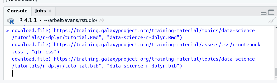
- Run the following code:
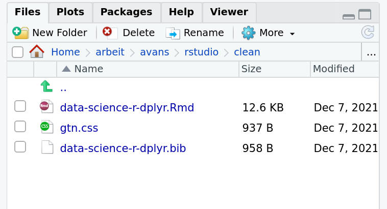
download.file("https://training.galaxyproject.org/training-material/topics/data-science/tutorials/r-dplyr/data-science-r-dplyr.Rmd", "data-science-r-dplyr.Rmd") download.file("https://training.galaxyproject.org/training-material/assets/css/r-notebook.css", "gtn.css") download.file("https://training.galaxyproject.org/training-material/topics/data-science/tutorials/r-dplyr/tutorial.bib", "data-science-r-dplyr.bib")- Double click the RMarkdown document that appears in the list of files on the right.
Downloading the notebook
- Right click this link: tutorial.Rmd
- Save Link As...
Alternative Formats
- This tutorial is also available as a Jupyter Notebook (With Solutions), Jupyter Notebook (Without Solutions)
Hands On: Learning with RMarkdown in RStudioLearning with RMarkdown is a bit different than you might be used to. Instead of copying and pasting code from the GTN into a document you’ll instead be able to run the code directly as it was written, inside RStudio! You can now focus just on the code and reading within RStudio.
Load the notebook if you have not already, following the tip box at the top of the tutorial
Open it by clicking on the
.Rmdfile in the file browser (bottom right)
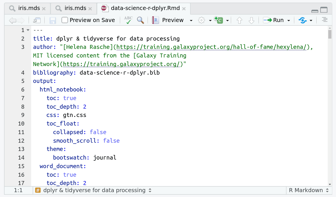
The RMarkdown document will appear in the document viewer (top left)
You’re now ready to view the RMarkdown notebook! Each notebook starts with a lot of metadata about how to build the notebook for viewing, but you can ignore this for now and scroll down to the content of the tutorial.
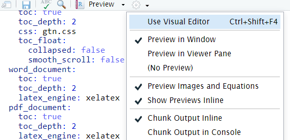
You can switch to the visual mode which is way easier to read - just click on the gear icon and select
Use Visual Editor.
You’ll see codeblocks scattered throughout the text, and these are all runnable snippets that appear like this in the document:
And you have a few options for how to run them:
- Click the green arrow
- ctrl+enter
Using the menu at the top to run all
When you run cells, the output will appear below in the Console. RStudio essentially copies the code from the RMarkdown document, to the console, and runs it, just as if you had typed it out yourself!
One of the best features of RMarkdown documents is that they include a very nice table browser which makes previewing results a lot easier! Instead of needing to use
headevery time to preview the result, you get an interactive table browser for any step which outputs a table.
dplyr (Wickham et al. 2021) is a powerful R-package to transform and summarize tabular data with rows and columns. It is part of a group of packages (including ggplot2) called the tidyverse (Wickham et al. 2019), a collection of packages for data processing and visualisation. For further exploration please see the dplyr package vignette: Introduction to dplyr
CommentThis tutorial is significantly based on GenomicsClass/labs.
AgendaIn this tutorial, we will cover:
Why Is It Useful?
The package contains a set of functions (or “verbs”) that perform common data manipulation operations such as filtering for rows, selecting specific columns, re-ordering rows, adding new columns and summarizing data.
In addition, dplyr contains a useful function to perform another common task which is the “split-apply-combine” concept. We will discuss that in a little bit.
How Does It Compare To Using Base Functions R?
If you are familiar with R, you are probably familiar with base R functions such as split(), subset(), apply(), sapply(), lapply(), tapply() and aggregate(). Compared to base functions in R, the functions in dplyr are easier to work with, are more consistent in the syntax and are targeted for data analysis around tibbles, instead of just vectors.
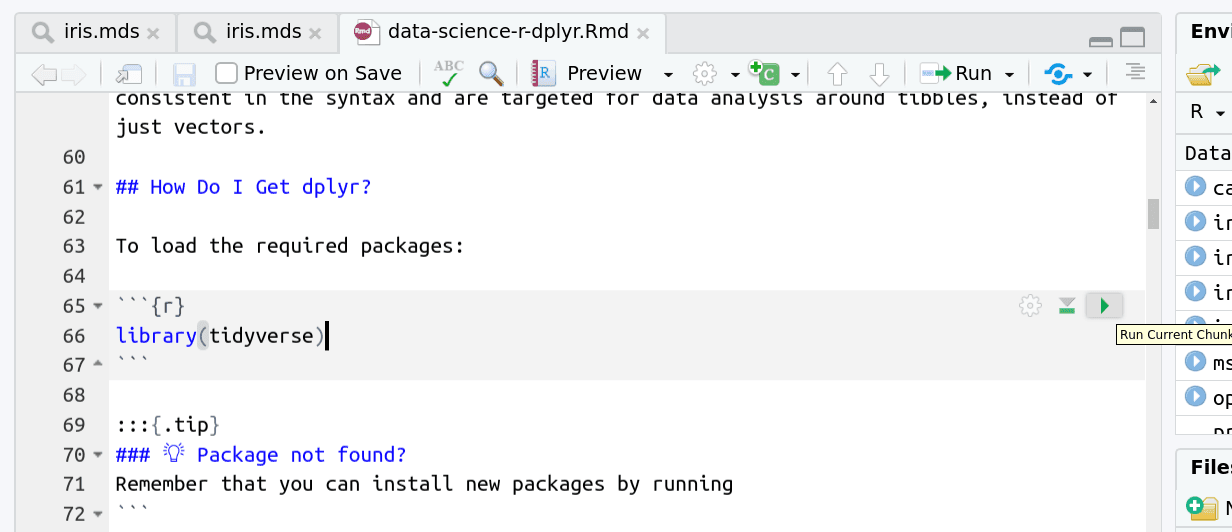
How Do I Get dplyr?
To load the required packages:
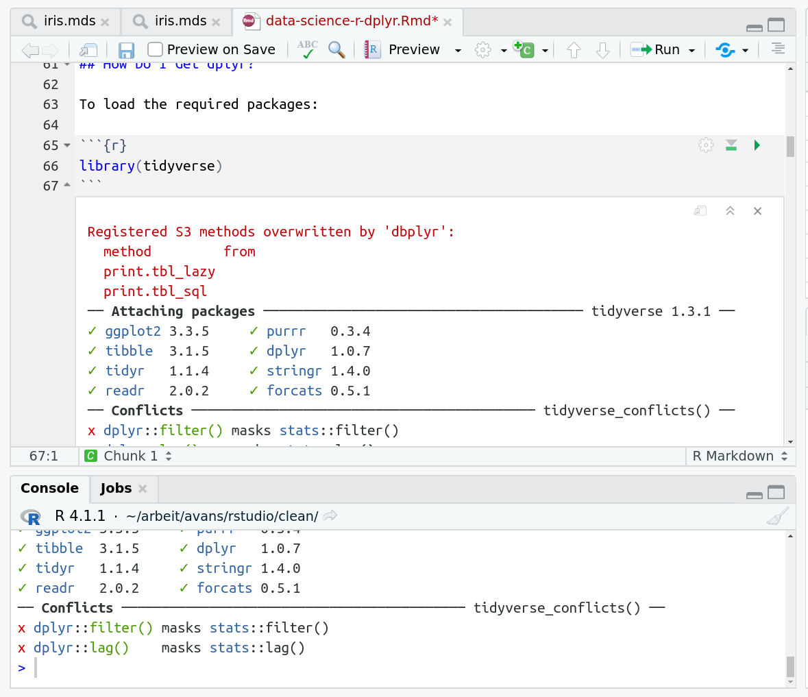
library(tidyverse)
Remember that you can install new packages by running
install.packages("tidyverse")Or by using the Install button on the RStudio Packages interface
Here we’ve imported the entire suite of tidyverse packages. We’ll specifically be using:
| Package | Use |
|---|---|
readr |
This provides the read_csv function which is identical to read.csv except it returns a tibble |
dplyr |
All of the useful functions we’ll be covering are part of dplyr |
magrittr |
A dependency of dplyr that provides the %>% operator |
ggplot2 |
The famous plotting library which we’ll use at the very end to plot our aggregated data. |
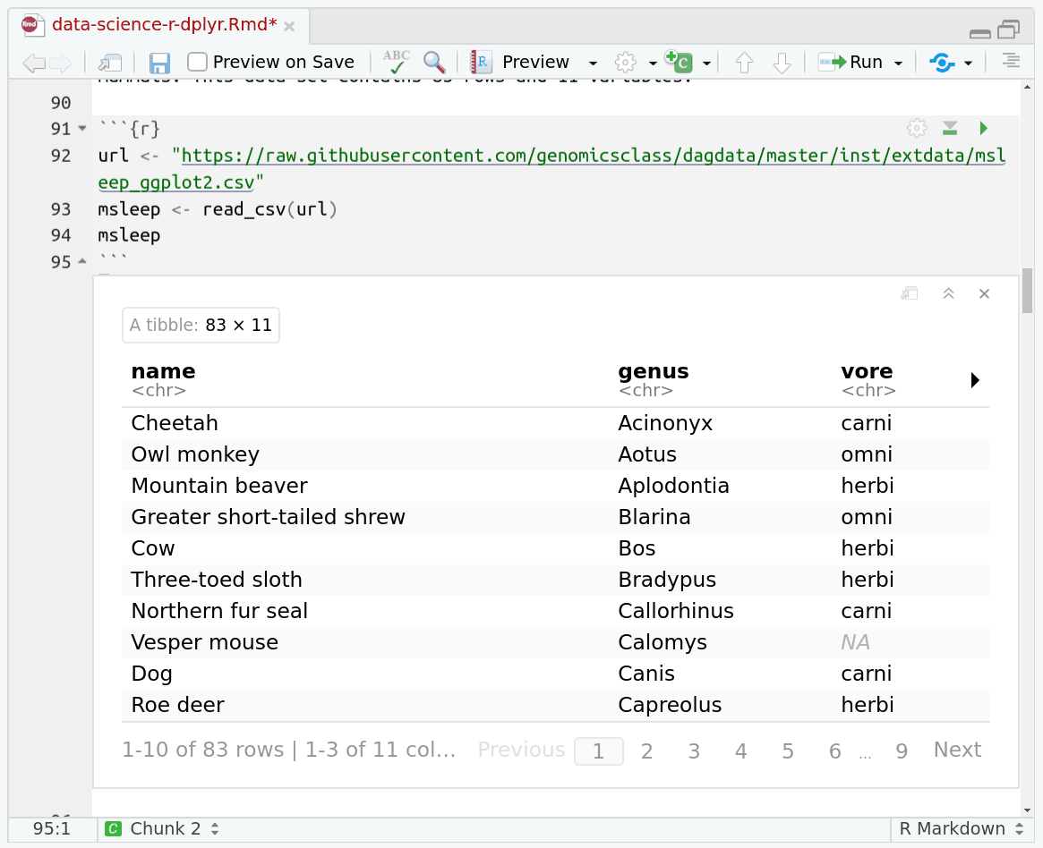
Data: Mammals Sleep
The msleep (mammals sleep) data set contains the sleep times and weights for a set of mammals. This data set contains 83 rows and 11 variables.
url <- "https://raw.githubusercontent.com/genomicsclass/dagdata/master/inst/extdata/msleep_ggplot2.csv"
msleep <- read_csv(url)
head(msleep)
The columns (in order) correspond to the following:
| column name | Description |
|---|---|
| name | common name |
| genus | taxonomic rank |
| vore | carnivore, omnivore or herbivore? |
| order | taxonomic rank |
| conservation | the conservation status of the mammal |
| sleep_total | total amount of sleep, in hours |
| sleep_rem | rem sleep, in hours |
| sleep_cycle | length of sleep cycle, in hours |
| awake | amount of time spent awake, in hours |
| brainwt | brain weight in kilograms |
| bodywt | body weight in kilograms |
Compare the above output with the more traditional read.csv that is built into R
dfmsleep <- read.csv(url)
head(dfmsleep)
This is a “data frame” and was the basis of data processing for years in R, and is still quite commonly used! But notice how dplyr has a much prettier and more consice output. This is what is called a tibble (like a table). We can immediately see metadata about the table, the separator that was guessed for us, what datatypes each column was (dbl or chr), how many rows and columns we have, etc. The tibble works basically exactly like a data frame except it has a lot of features to integrate nicely with the dplyr package.
That said, all of the functions below you will learn about work equally well with data frames and tibbles, but tibbles will save you from filling your screen with hundreds of rows by automatically truncating large tables unless you specifically request otherwise.
Important dplyr Verbs To Remember
| dplyr verbs | Description | SQL Equivalent Operation |
|---|---|---|
select() |
select columns | SELECT |
filter() |
filter rows | WHERE |
arrange() |
re-order or arrange rows | ORDER BY |
mutate() |
create new columns | SELECT x, x*2 ... |
summarise() |
summarise values | n/a |
group_by() |
allows for group operations in the “split-apply-combine” concept | GROUP BY |
dplyr Verbs In Action
The two most basic functions are select() and filter(), which selects columns and filters rows respectively.
Pipe Operator: %>%
Before we go any further, let’s introduce the pipe operator: %>%. dplyr imports this operator from another package (magrittr).This operator allows you to pipe the output from one function to the input of another function. Instead of nesting functions (reading from the inside to the outside), the idea of piping is to read the functions from left to right. This is a lot more like how you would write a bash data processing pipeline and can be a lot more readable and intuitive than the nested version.
Here’s is the more old fashioned way of writing the equivalent code:
head(select(msleep, name, sleep_total))
Now in this case, we will pipe the msleep tibble to the function that will select two columns (name and sleep_total) and then pipe the new tibble to the function head(), which will return the head of the new tibble.
msleep %>% select(name, sleep_total) %>% head(2)
QuestionHow would you rewrite the following code to use the pipe operator?
prcomp(tail(read.csv("file.csv"), 10))Just read from inside to outside, starting with the innermost
()and use%>%between each step.read.csv("file.csv") %>% tail(10) %>% prcomp()
Selecting Columns Using select()
Select a set of columns: the name and the sleep_total columns.
msleep %>% select(name, sleep_total)
To select all the columns except a specific column, use the “-“ (subtraction) operator (also known as negative indexing):
msleep %>% select(-name)
To select a range of columns by name, use the “:” (colon) operator:
msleep %>% select(name:order)
To select all columns that start with the character string “sl”, use the function starts_with():
msleep %>% select(starts_with("sl"))
Some additional options to select columns based on a specific criteria include:
| Function | Usage |
|---|---|
ends_with() |
Select columns that end with a character string |
contains() |
Select columns that contain a character string |
matches() |
Select columns that match a regular expression |
one_of() |
Select column names that are from a group of names |
Selecting Rows Using filter()
Filter the rows for mammals that sleep a total of more than 16 hours.
msleep %>% filter(sleep_total >= 16)
Filter the rows for mammals that sleep a total of more than 16 hours and have a body weight of greater than 1 kilogram.
msleep %>% filter(sleep_total >= 16, bodywt >= 1)
Filter the rows for mammals in the Perissodactyla and Primates taxonomic order
msleep %>% filter(order %in% c("Perissodactyla", "Primates"))
You can use the boolean operators (e.g. >, <, >=, <=, !=, %in%) to create the logical tests.
Arrange Or Re-order Rows Using arrange()
To arrange (or re-order) rows by a particular column, such as the taxonomic order, list the name of the column you want to arrange the rows by:
msleep %>% arrange(order) %>% select(order, genus, name)
Now we will select three columns from msleep, arrange the rows by the taxonomic order and then arrange the rows by sleep_total. Finally, show the final tibble:
msleep %>%
    select(name, order, sleep_total) %>%
    arrange(order, sleep_total)
Same as above, except here we filter the rows for mammals that sleep for 16 or more hours, instead of showing the whole tibble:
msleep %>%
    select(name, order, sleep_total) %>%
    arrange(order, sleep_total) %>%
    filter(sleep_total >= 16)
Something slightly more complicated: same as above, except arrange the rows in the sleep_total column in a descending order. For this, use the function desc()
msleep %>%
    select(name, order, sleep_total) %>%
    arrange(order, desc(sleep_total)) %>%
    filter(sleep_total >= 16)
Create New Columns Using mutate()
The mutate() function will add new columns to the tibble. Create a new column called rem_proportion, which is the ratio of rem sleep to total amount of sleep.
msleep %>%
  mutate(rem_proportion = sleep_rem / sleep_total) %>%
  select(starts_with("sl"), rem_proportion)
You can many new columns using mutate (separated by commas). Here we add a second column called bodywt_grams which is the bodywt column in grams.
msleep %>%
    mutate(rem_proportion = sleep_rem / sleep_total,
           bodywt_grams = bodywt * 1000) %>%
    select(sleep_total, sleep_rem, rem_proportion, bodywt, bodywt_grams)
Create summaries of the tibble using summarise()
The summarise() function will create summary statistics for a given column in the tibble such as finding the mean. For example, to compute the average number of hours of sleep, apply the mean() function to the column sleep_total and call the summary value avg_sleep.
msleep %>%
    summarise(avg_sleep = mean(sleep_total))
There are many other summary statistics you could consider such sd(), min(), max(), median(), sum(), n() (returns the length of vector), first() (returns first value in vector), last() (returns last value in vector) and n_distinct() (number of distinct values in vector).
msleep %>%
    summarise(avg_sleep = mean(sleep_total),
              min_sleep = min(sleep_total),
              max_sleep = max(sleep_total),
              total = n())
Group operations using group_by()
The group_by() verb is an important function in dplyr. As we mentioned before it’s related to concept of “split-apply-combine”. We literally want to split the tibble by some variable (e.g. taxonomic order), apply a function to the individual tibbles and then combine the output.
Let’s do that: split the msleep tibble by the taxonomic order, then ask for the same summary statistics as above. We expect a set of summary statistics for each taxonomic order.
msleep %>%
    group_by(order) %>%
    summarise(avg_sleep = mean(sleep_total),
              min_sleep = min(sleep_total),
              max_sleep = max(sleep_total),
              total = n())
ggplot2
Most people want to slice and dice their data before plotting, so let’s demonstrate that quickly by plotting our last dataset.
library(ggplot2)
msleep %>%
    group_by(order) %>%
    summarise(avg_sleep = mean(sleep_total),
              min_sleep = min(sleep_total),
              max_sleep = max(sleep_total),
              total = n()) %>%
    ggplot() + geom_point(aes(x=min_sleep, y=max_sleep, colour=order))
Notice how we can just keep piping our data together, this makes it incredibly easier to experiment and play around with our data and test out what filtering or summarisation we want and how that will plot in the end. If we wanted, or if the data processing is an especially computationally expensive step, we could save it to an intermediate variable before playing around with plotting options, but in the case of this small dataset that’s probably not necessary.
You've Finished the Tutorial
Key points
Dplyr and tidyverse make it a lot easier to process data
The functions for selecting data are a lot easier to understand than R’s built in alternatives.
Frequently Asked Questions
Have questions about this tutorial? Have a look at the available FAQ pages and support channelsReferences
- Wickham, H., M. Averick, J. Bryan, W. Chang, L. D. A. McGowan et al., 2019 Welcome to the tidyverse. Journal of Open Source Software 4: 1686. 10.21105/joss.01686
- Wickham, H., R. François, L. Henry, and K. Müller, 2021 dplyr: A Grammar of Data Manipulation. R package version 1.0.7. https://CRAN.R-project.org/package=dplyr
Feedback
Did you use this material as an instructor? Feel free to give us feedback on how it went.
Did you use this material as a learner or student? Click the form below to leave feedback.

Citing this Tutorial
- Helena Rasche, avans-atgm, dplyr & tidyverse for data processing (Galaxy Training Materials). https://training.galaxyproject.org/training-material/topics/data-science/tutorials/r-dplyr/tutorial.html Online; accessed TODAY
- Hiltemann, Saskia, Rasche, Helena et al., 2023 Galaxy Training: A Powerful Framework for Teaching! PLOS Computational Biology 10.1371/journal.pcbi.1010752
- Batut et al., 2018 Community-Driven Data Analysis Training for Biology Cell Systems 10.1016/j.cels.2018.05.012
@misc{data-science-r-dplyr,
author = "Helena Rasche and avans-atgm",
	title = "dplyr & tidyverse for data processing (Galaxy Training Materials)",
	year = "",
	month = "",
	day = "",
	url = "\url{https://training.galaxyproject.org/training-material/topics/data-science/tutorials/r-dplyr/tutorial.html}",
	note = "[Online; accessed TODAY]"
}
@article{Hiltemann_2023,
	doi = {10.1371/journal.pcbi.1010752},
	url = {https://doi.org/10.1371%2Fjournal.pcbi.1010752},
	year = 2023,
	month = {jan},
	publisher = {Public Library of Science ({PLoS})},
	volume = {19},
	number = {1},
	pages = {e1010752},
	author = {Saskia Hiltemann and Helena Rasche and Simon Gladman and Hans-Rudolf Hotz and Delphine Larivi{\`{e}}re and Daniel Blankenberg and Pratik D. Jagtap and Thomas Wollmann and Anthony Bretaudeau and Nadia Gou{\'{e}} and Timothy J. Griffin and Coline Royaux and Yvan Le Bras and Subina Mehta and Anna Syme and Frederik Coppens and Bert Droesbeke and Nicola Soranzo and Wendi Bacon and Fotis Psomopoulos and Crist{\'{o}}bal Gallardo-Alba and John Davis and Melanie Christine Föll and Matthias Fahrner and Maria A. Doyle and Beatriz Serrano-Solano and Anne Claire Fouilloux and Peter van Heusden and Wolfgang Maier and Dave Clements and Florian Heyl and Björn Grüning and B{\'{e}}r{\'{e}}nice Batut and},
	editor = {Francis Ouellette},
	title = {Galaxy Training: A powerful framework for teaching!},
	journal = {PLoS Comput Biol}
}
Funding
These individuals or organisations provided funding support for the development of this resource
Congratulations on successfully completing this tutorial!Do you want to extend your knowledge?Follow one of our recommended follow-up trainings: