Advanced Python
| Author(s) |
|
| Reviewers |
|
OverviewQuestions:
Objectives:
How can I analyze data using Python with Numpy and Pandas?
Requirements:
Use the scientific libraries pandas and numpy to explore tabular datasets
Calculate basic statistics about datasets and columns
Time estimation: 3 hoursLevel: Intermediate IntermediateSupporting Materials:Published: Nov 8, 2021Last modification: Oct 15, 2024License: Tutorial Content is licensed under Creative Commons Attribution 4.0 International License. The GTN Framework is licensed under MITpurl PURL: https://gxy.io/GTN:T00081rating Rating: 5.0 (0 recent ratings, 1 all time)version Revision: 7
Best viewed in a Jupyter NotebookThis tutorial is best viewed in a Jupyter notebook! You can load this notebook one of the following ways
Run on the GTN with JupyterLite (in-browser computations)
Launching the notebook in Jupyter in Galaxy
- Instructions to Launch JupyterLab
- Open a Terminal in JupyterLab with File -> New -> Terminal
- Run
wget https://training.galaxyproject.org/training-material/topics/data-science/tutorials/python-advanced-np-pd/data-science-python-advanced-np-pd.ipynb- Select the notebook that appears in the list of files on the left.
Downloading the notebook
- Right click one of these links: Jupyter Notebook (With Solutions), Jupyter Notebook (Without Solutions)
- Save Link As..
In this lesson, we will be using Python 3 with some of its most popular scientific libraries. This tutorial assumes that the reader is familiar with the fundamentals of the Python programming language, as well as, how to run Python programs using Galaxy. Otherwise, it is advised to follow the “Introduction to Python” tutorial available in the same platform. We will be using JupyterNotebook, a Python interpreter that comes with everything we need for the lesson. Please note: JupyterNotebook is only currently available on the usegalaxy.eu and usegalaxy.org sites.
CommentThis tutorial is significantly based on the Carpentries Programming with Python and Plotting and Programming in Python, which is licensed CC-BY 4.0.
Adaptations have been made to make this work better in a GTN/Galaxy environment.
AgendaIn this tutorial, we will cover:
Analyze data using numpy
NumPy is a python library and it stands for Numerical Python. In general, you should use this library when you want to perform operations and manipulate numerical data, especially if you have matrices or arrays. To tell Python that we’d like to start using NumPy, we need to import it:
import numpy as np
A Numpy array contains one or more elements of the same type. To examine the basic functions of the library, we will create an array of random data. These data will correspond to arthritis patients’ inflammation. The rows are the individual patients, and the columns are their daily inflammation measurements. We will use the random.randint() function. It has 4 arguments as inputs randint(low, high=None, size=None, dtype=int). low nad high specify the limits of the random number generator. size determines the shape of the array and it can be an integer or a tuple.
np.random.seed(2021)  #create reproducible work
random_data = np.random.randint(1, 25, size=(50,70))
If we want to check the data have been loaded, we can print the variable’s value:
print(random_data)
Now that the data are in memory, we can manipulate them. First, let’s ask what type of thing data refers to:
print(type(random_data))
The output tells us that data currently refers to an N-dimensional array, the functionality for which is provided by the NumPy library. These data correspond to arthritis patients’ inflammation. The rows are the individual patients, and the columns are their daily inflammation measurements.
The type function will only tell you that a variable is a NumPy array but won’t tell you the type of thing inside the array. We can find out the type of the data contained in the NumPy array.
print(random_data.dtype)
This tells us that the NumPy array’s elements are integer numbers.
With the following command, we can see the array’s shape:
print(random_data.shape)
The output tells us that the data array variable contains 50 rows and 70 columns. When we created the variable random_data to store our arthritis data, we did not only create the array; we also created information about the array, called members or attributes. This extra information describes random_data in the same way an adjective describes a noun. random_data.shape is an attribute of random_data which describes the dimensions of random_data.
If we want to get a single number from the array, we must provide an index in square brackets after the variable name, just as we do in math when referring to an element of a matrix. Our data has two dimensions, so we will need to use two indices to refer to one specific value:
print('first value in data:', random_data[0, 0])
print('middle value in data:', random_data[25, 35])
The expression random_data[25, 35] accesses the element at row 25, column 35. While this expression may not surprise you, random_data[0, 0] might. Programming languages like Fortran, MATLAB and R start counting at 1 because that’s what human beings have done for thousands of years. Languages in the C family (including C++, Java, Perl, and Python) count from 0 because it represents an offset from the first value in the array (the second value is offset by one index from the first value). As a result, if we have an M×N array in Python, its indices go from 0 to M-1 on the first axis and 0 to N-1 on the second.
Slicing data An index like [25, 35] selects a single element of an array, but we can select whole sections as well, using slicing the same way as previously with the strings. For example, we can select the first ten days (columns) of values for the first four patients (rows) like this:
print(random_data[0:4, 0:10])
We don’t have to include the upper and lower bound on the slice. If we don’t include the lower bound, Python uses 0 by default; if we don’t include the upper, the slice runs to the end of the axis, and if we don’t include either (i.e., if we use ‘:’ on its own), the slice includes everything:
small = random_data[:3, 36:]
print('small is:')
print(small)
The above example selects rows 0 through 2 and columns 36 through to the end of the array.
Process the data
NumPy has several useful functions that take an array as input to perform operations on its values. If we want to find the average inflammation for all patients on all days, for example, we can ask NumPy to compute random_data’s mean value:
print(np.mean(random_data))
Let’s use three other NumPy functions to get some descriptive values about the dataset. We’ll also use multiple assignment, a convenient Python feature that will enable us to do this all in one line.
maxval, minval, stdval = np.max(random_data), np.min(random_data), np.std(random_data)

print('maximum inflammation:', maxval)
print('minimum inflammation:', minval)
print('standard deviation:', stdval)
How did we know what functions NumPy has and how to use them? If you are working in IPython or in a Jupyter Notebook, there is an easy way to find out. If you type the name of something followed by a dot, then you can use tab completion (e.g. type np. and then press Tab) to see a list of all functions and attributes that you can use. After selecting one, you can also add a question mark (e.g. np.cumprod?), and IPython will return an explanation of the method! This is the same as doing help(np.cumprod).
When analyzing data, though, we often want to look at variations in statistical values, such as the maximum inflammation per patient or the average inflammation per day. One way to do this is to create a new temporary array of the data we want, then ask it to do the calculation:
patient_0 = random_data[0, :] # 0 on the first axis (rows), everything on the second (columns)
print('maximum inflammation for patient 0:', np.max(patient_0))
What if we need the maximum inflammation for each patient over all days (as in the next diagram on the left) or the average for each day (as in the diagram on the right)? As the diagram below shows, we want to perform the operation across an axis:
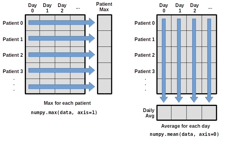
To support this functionality, most array functions allow us to specify the axis we want to work on. If we ask for the average across axis 0 (rows in our 2D example), we get:
print(np.mean(random_data, axis=0))
As a quick check, we can ask this array what its shape is:
print(np.mean(random_data, axis=0).shape)
The expression (70,) tells us we have an N×1 vector, so this is the average inflammation per day for all patients. If we average across axis 1 (columns in our 2D example), we get the average inflammation per patient across all days.:
print(np.mean(random_data, axis=1))
Stacking arrays
Arrays can be concatenated and stacked on top of one another, using NumPy’s vstack and hstack functions for vertical and horizontal stacking, respectively.
import numpy as np

A = np.array([[1,2,3], [4,5,6], [7, 8, 9]])
print('A = ')
print(A)

B = np.hstack([A, A])
print('B = ')
print(B)

C = np.vstack([A, A])
print('C = ')
print(C)
Remove NaN values
Sometimes there are missing values in an array, that could make it difficult to perform operations on it. To remove the NaN you must first find their indexes and then replace them. The following example replaces them with 0.
a = array([[1, 2, 3], [0, 3, NaN]])
print(a)
a[np.isnan(a)] = 0
print(a)
Question: Selecting and stacking arraysWrite some additional code that slices the first and last columns of A, and stacks them into a 3x2 array. Make sure to print the results to verify your solution.
A ‘gotcha’ with array indexing is that singleton dimensions are dropped by default. That means
A[:, 0]is a one dimensional array, which won’t stack as desired. To preserve singleton dimensions, the index itself can be a slice or array. For example,A[:, :1]returns a two dimensional array with one singleton dimension (i.e. a column vector).D = np.hstack((A[:, :1], A[:, -1:])) print('D = ') print(D)
Question: Selecting with conditionalsGiven the followind array
A, keep only the elements that are lower that0.05.A = np.array([0.81, 0.025, 0.15, 0.67, 0.01])A = A[A<0.05]
Use pandas to work with dataframes
Pandas (pandas development team 2020, Wes McKinney 2010 ) is a widely-used Python library for statistics, particularly on tabular data. If you are familiar with R dataframes, then this is the library that integrates this functionality. A dataframe is a 2-dimensional table with indexes and column names. The indexes indicate the difference in rows, while the column names indicate the difference in columns. You will see later that these two features are useful when you’re manipulating your data. Each column can contain different data types.
Load it with import pandas as pd. The alias pd is commonly used for pandas.
import pandas as pd
There are many ways to create a pandas dataframe. For example you can use a numpy array as input.
data = np.array([['','Col1','Col2'],
                ['Row1',1,2],
                ['Row2',3,4]])

print(pd.DataFrame(data=data[1:,1:],
                  index=data[1:,0],
                  columns=data[0,1:]))
For the purposes of this tutorial, we will use a file with the annotated differentially expressed genes that was produced in the Reference-based RNA-Seq data analysis tutorial
We can read a tabular file with pd.read_csv. The first argument is the filepath of the file to be read. The sep argument refers to the symbol used to separate the data into different columns. You can check the rest of the arguments using the help() function.
data = pd.read_csv("https://zenodo.org/record/3477564/files/annotatedDEgenes.tabular", sep = "\t")
print(data)
The columns in a dataframe are the observed variables, and the rows are the observations. Pandas uses backslash \ to show wrapped lines when output is too wide to fit the screen.
Explore the data
You can use index_col to specify that a column’s values should be used as row headings.
By default row indexes are numbers, but we could use a column of the data. To pass the name of the column to read_csv, you can use its index_col parameter. Be careful though, because the row indexes must be unique for each row.
data = pd.read_csv("https://zenodo.org/record/3477564/files/annotatedDEgenes.tabular", sep = "\t", index_col = 'GeneID')
print(data)
You can use the DataFrame.info() method to find out more about a dataframe.
data.info()
We learn that this is a DataFrame. It consists of 130 rows and 12 columns. None of the columns contains any missing values. 6 columns contain 64-bit floating point float64 values, 2 contain 64-bit integer int64 values and 4 contain character object values. It uses 13.2KB of memory.
The DataFrame.columns variable stores information about the dataframe’s columns.
Note that this is an attribute, not a method. (It doesn’t have parentheses.) Called a member variable, or just member.
print(data.columns)
You could use DataFrame.T to transpose a dataframe. The Transpose (written .T) doesn’t copy the data, just changes the program’s view of it. Like columns, it is a member variable.
print(data.T)
You can use DataFrame.describe() to get summary statistics about the data. DataFrame.describe() returns the summary statistics of only the columns that have numerical data. All other columns are ignored, unless you use the argument include='all'. Depending on the data type of each column, the statistics that can’t be calculated are replaced with the value NaN.
print(data.describe(include='all'))
Question: Using pd.head and pd.tailAfter reading the data, use
help(data.head)andhelp(data.tail)to find out whatDataFrame.headandDataFrame.taildo. a. What method call will display the first three rows of the data? b. What method call will display the last three columns of this data? (Hint: you may need to change your view of the data.)a. We can check out the first five rows of the data by executing
data.head()(allowing us to view the head of the DataFrame). We can specify the number of rows we wish to see by specifying the parameternin our call todata.head(). To view the first three rows, execute:data.head(n=3)
Base mean log2(FC) StdErr Wald-Stats P-value P-adj Chromosome Start End Strand Feature Gene name GeneID FBgn0039155 1086.974295 -4.148450 0.134949 -30.740913 1.617357e-207 1.387207e-203 chr3R 24141394 24147490 + protein_coding Kal1 FBgn0003360 6409.577128 -2.999777 0.104345 -28.748637 9.419922e-182 4.039734e-178 chrX 10780892 10786958 - protein_coding sesB FBgn0026562 65114.840564 -2.380164 0.084327 -28.225437 2.850430e-175 8.149380e-172 chr3R 26869237 26871995 - protein_coding BM-40-SPARC b. To check out the last three rows, we would use the command,
data.tail(n=3), analogous tohead()used above. However, here we want to look at the last three columns so we need to change our view and then usetail(). To do so, we create a new DataFrame in which rows and columns are switched:data_flipped = data.TWe can then view the last three columns of the data by viewing the last three rows of data_flipped:
data_flipped.tail(n=3)| GeneID | FBgn0039155 | FBgn0003360 | FBgn0026562 | FBgn0025111 | FBgn0029167 | FBgn0039827 | FBgn0035085 | FBgn0034736 | FBgn0264475 | FBgn0000071 | … | FBgn0264343 | FBgn0038237 | FBgn0020376 | FBgn0028939 | FBgn0036560 | FBgn0035710 | FBgn0035523 | FBgn0038261 | FBgn0039178 | FBgn0034636 | | —- | —- | —- | —- | —- | —- | —- | —- | —- | —- | —- | —- | —- | —- | —- | —- | —- | —- | —- | —- | —- | —- | | Strand | + | - | - | - | + | + | + | + | + | + | … | + | - | + | + | + | - | + | + | + | - | | Feature | protein_coding | protein_coding | protein_coding | protein_coding | protein_coding | protein_coding | protein_coding | protein_coding | lincRNA | protein_coding | … | protein_coding | protein_coding | protein_coding | protein_coding | protein_coding | protein_coding | protein_coding | protein_coding | protein_coding | protein_coding | | Gene name | Kal1 | sesB | BM-40-SPARC | Ant2 | Hml | CG1544 | CG3770 | CG6018 | CR43883 | Ama | … | CG43799 | Pde6 | Sr-CIII | NimC2 | CG5895 | SP1173 | CG1311 | CG14856 | CG6356 | CG10440 |
Question: Saving in a csv fileAs well as the
read_csvfunction for reading data from a file, Pandas provides ato_csvfunction to write dataframes to files. Applying what you’ve learned about reading from files, write one of your dataframes to a file calledprocessed.csv. You can usehelpto get information on how to useto_csv.data_flipped.to_csv('processed.csv')
- Note about Pandas DataFrames/Series
A DataFrame is a collection of Series; The DataFrame is the way Pandas represents a table, and Series is the data-structure Pandas use to represent a column.
Pandas is built on top of the Numpy library, which in practice means that most of the methods defined for Numpy Arrays apply to Pandas Series/DataFrames.
What makes Pandas so attractive is the powerful interface to access individual records of the table, proper handling of missing values, and relational-databases operations between DataFrames.
Select data
To access a value at the position [i,j] of a DataFrame, we have two options, depending on what is the meaning of i in use. Remember that a DataFrame provides an index as a way to identify the rows of the table; a row, then, has a position inside the table as well as a label, which uniquely identifies its entry in the DataFrame.
You can use DataFrame.iloc[..., ...] to select values by their (entry) position and basically specify location by numerical index analogously to 2D version of character selection in strings.
print(data.iloc[0, 0])
You can also use DataFrame.loc[..., ...] to select values by their (entry) label and basically specify location by row name analogously to 2D version of dictionary keys.
print(data.loc["FBgn0039155", "Base mean"])
You can use Python’s usual slicing notation, to select all or a subset of rows and/or columns. For example, the following code selects all the columns of the row "FBgn0039155".
print(data.loc["FBgn0039155", :])
Which would get the same result as printing data.loc["FBgn0039155"] (without a second index).
You can select multiple columns or rows using DataFrame.loc and a named slice or Dataframe.iloc and the numbers corresponding to the rows and columns.
print(data.loc['FBgn0003360':'FBgn0029167', 'Base mean':'Wald-Stats'])
print(data.iloc[1:4 , 0:3])
- Note the difference between the 2 outputs.
When choosing or transitioning between loc and iloc, you should keep in mind that the two methods use slightly different indexing schemes.
iloc uses the Python stdlib indexing scheme, where the first element of the range is included and the last one excluded. So 0:10 will select entries 0,...,9. loc, meanwhile, indexes inclusively. So 0:10 will select entries 0,...,10.
This is particularly confusing when the DataFrame index is a simple numerical list, e.g. 0,...,1000. In this case df.iloc[0:1000] will return 1000 entries, while df.loc[0:1000] return 1001 of them! To get 1000 elements using loc, you will need to go one lower and ask for df.loc[0:999].
The result of slicing is a new dataframe and can be used in further operations. All the statistical operators that work on entire dataframes work the same way on slices. E.g., calculate max of a slice.
print(data.loc['FBgn0003360':'FBgn0029167', 'Base mean'].max())
Use conditionals to select data
You can use conditionals to select data. A comparison is applied element by element and returns a similarly-shaped dataframe of True and False. The last one can be used as a mask to subset the original dataframe. The following example creates a new dataframe consisting only of the columns ‘P-adj’ and ‘Gene name’, then keeps the rows that comply with the expression 'P-adj' < 0.000005
subset = data.loc[:, ['P-adj', 'Gene name']]
print(subset)
mask = subset.loc[:, 'P-adj'] < 0.000005
new_data = subset[mask]
print(new_data)
If we have not had specified the column, that the expression should be applied to, then it would have been applied to the entire dataframe. But the dataframe contains different type of data. In that case, an error would occur.
Consider the following example of a dataframe consisting only of numerical data. The expression and the mask would be normally applied to the data and the mask would return NaN for the data that don’t comply with the expression.
subset = data.loc[:, ['StdErr',	'Wald-Stats', 'P-value', 'P-adj']]
mask = subset < 0.05
new_data = subset[mask]
print(new_data)
This is very useful because NaNs are ignored by operations like max, min, average, etc.
print(new_data.describe())
Question: Manipulating dataframesExplain what each line in the following short program does: what is in first, second, etc.?
first = pd.read_csv("https://zenodo.org/record/3477564/files/annotatedDEgenes.tabular", sep = "\t", index_col = 'GeneID') second = first[first['log2(FC)'] > 0 ] third = second.drop('FBgn0025111') fourth = third.drop('StdErr', axis = 1) fourth.to_csv('result.csv')Let’s go through this piece of code line by line.
first = pd.read_csv("https://zenodo.org/record/3477564/files/annotatedDEgenes.tabular", sep = "\t", index_col = 'GeneID')This line loads the data into a dataframe called first. The
index_col='GeneID'parameter selects which column to use as the row labels in the dataframe.second = first[first['log2(FC)'] > 0 ]This line makes a selection: only those rows of first for which the ‘log2(FC)’ column contains a positive value are extracted. Notice how the Boolean expression inside the brackets is used to select only those rows where the expression is true.
third = second.drop('FBgn0025111')As the syntax suggests, this line drops the row from second where the label is ‘FBgn0025111’. The resulting dataframe third has one row less than the original dataframe second.
fourth = third.drop('StdErr', axis = 1)Again we apply the drop function, but in this case we are dropping not a row but a whole column. To accomplish this, we need to specify also the axis parameter.
fourth.to_csv('result.csv')The final step is to write the data that we have been working on to a csv file. Pandas makes this easy with the
to_csv()function. The only required argument to the function is the filename. Note that the file will be written in the directory from which you started the Jupyter or Python session.
Question: Finding min-max indexesExplain in simple terms what
idxminandidxmaxdo in the short program below. When would you use these methods?data = pd.read_csv("https://zenodo.org/record/3477564/files/annotatedDEgenes.tabular", sep = "\t", index_col = 'GeneID') print(data['Base mean'].idxmin()) print(data['Base mean'].idxmax())
idxminwill return the index value corresponding to the minimum; idxmax will do the same for the maximum value.You can use these functions whenever you want to get the row index of the minimum/maximum value and not the actual minimum/maximum value.
Output: FBgn0063667 FBgn0026562
Question: Selecting with conditionalsAssume Pandas has been imported and the previous dataset has been loaded. Write an expression to select each of the following: a. P-value of each gene b. all the information of gene
FBgn0039178c. the information of all genes that belong to chromosomechr3Ra.
data['P-value']b.data.loc['FBgn0039178', :]c.data[data['Chromosome'] == 'chr3R']
Group-by and analyze the data
Many data analysis tasks can be approached using the “split-apply-combine” paradigm: split the data into groups, apply some analysis to each group, and then combine the results.
Pandas makes this very easy through the use of the groupby() method, which splits the data into groups. When the data is grouped in this way, the aggregate method agg() can be used to apply an aggregating or summary function to each group.
summarised_data = data.groupby('Chromosome').agg({'Base mean':'first',
                             'log2(FC)': 'max'})
print(summarised_data)
There are a couple of things that should be noted. The agg() method accepts a dictionary as input that specifies the function to be applied to each column. The output is a new dataframe, that each row corresponds to one group. The output dataframe uses the grouping column as index. We could change the last one by simply using the reset_index() method.
summarised_data = data.groupby('Chromosome').agg({'Base mean':'first',
                                                  'log2(FC)': 'max'}).reset_index()
print(summarised_data)
Question: Finding the max of each groupUsing the same dataset, try to find the longest genes in each chromosome.
data['Gene Length'] = data['End'] - data['Start']
data.groupby('Chromosome').agg(max_length = ('Gene Length', 'max'))
Question: Grouping with multiple variablesUsing the same dataset, try to find how many genes are found on each strand of each chromosome.
You can group the data according to more than one column.
data.groupby(['Chromosome', 'Strand']).size()
Conclusion
This tutorial aims to serve as an introduction to data analysis using the Python programming language. We hope you feel more confident in Python!
You've Finished the Tutorial
Key points
Python has many libraries offering a variety of capabilities, which makes it popular for beginners, as well as, more experienced users
You can use scientific libraries like Numpy and Pandas to perform data analysis.
Frequently Asked Questions
Have questions about this tutorial? Have a look at the available FAQ pages and support channelsReferences
- McKinney, Wes, 2010 Data Structures for Statistical Computing in Python , pp. 56–61 in Proceedings of the 9th Python in Science Conference , edited by Stéfan van der Walt and Jarrod Millman. 10.25080/Majora-92bf1922-00a
- team, T. pandas development, 2020 pandas-dev/pandas: Pandas. 10.5281/zenodo.3509134
Feedback
Did you use this material as an instructor? Feel free to give us feedback on how it went.
Did you use this material as a learner or student? Click the form below to leave feedback.

Citing this Tutorial
- Maria Christina Maniou, Fotis E. Psomopoulos, carpentries, Advanced Python (Galaxy Training Materials). https://training.galaxyproject.org/training-material/topics/data-science/tutorials/python-advanced-np-pd/tutorial.html Online; accessed TODAY
- Hiltemann, Saskia, Rasche, Helena et al., 2023 Galaxy Training: A Powerful Framework for Teaching! PLOS Computational Biology 10.1371/journal.pcbi.1010752
- Batut et al., 2018 Community-Driven Data Analysis Training for Biology Cell Systems 10.1016/j.cels.2018.05.012
@misc{data-science-python-advanced-np-pd,
author = "Maria Christina Maniou and Fotis E. Psomopoulos and carpentries",
	title = "Advanced Python (Galaxy Training Materials)",
	year = "",
	month = "",
	day = "",
	url = "\url{https://training.galaxyproject.org/training-material/topics/data-science/tutorials/python-advanced-np-pd/tutorial.html}",
	note = "[Online; accessed TODAY]"
}
@article{Hiltemann_2023,
	doi = {10.1371/journal.pcbi.1010752},
	url = {https://doi.org/10.1371%2Fjournal.pcbi.1010752},
	year = 2023,
	month = {jan},
	publisher = {Public Library of Science ({PLoS})},
	volume = {19},
	number = {1},
	pages = {e1010752},
	author = {Saskia Hiltemann and Helena Rasche and Simon Gladman and Hans-Rudolf Hotz and Delphine Larivi{\`{e}}re and Daniel Blankenberg and Pratik D. Jagtap and Thomas Wollmann and Anthony Bretaudeau and Nadia Gou{\'{e}} and Timothy J. Griffin and Coline Royaux and Yvan Le Bras and Subina Mehta and Anna Syme and Frederik Coppens and Bert Droesbeke and Nicola Soranzo and Wendi Bacon and Fotis Psomopoulos and Crist{\'{o}}bal Gallardo-Alba and John Davis and Melanie Christine Föll and Matthias Fahrner and Maria A. Doyle and Beatriz Serrano-Solano and Anne Claire Fouilloux and Peter van Heusden and Wolfgang Maier and Dave Clements and Florian Heyl and Björn Grüning and B{\'{e}}r{\'{e}}nice Batut and},
	editor = {Francis Ouellette},
	title = {Galaxy Training: A powerful framework for teaching!},
	journal = {PLoS Comput Biol}
}
Funding
These individuals or organisations provided funding support for the development of this resource
Congratulations on successfully completing this tutorial!Do you want to extend your knowledge?Follow one of our recommended follow-up trainings: