Discovered over 40 years ago, alternative splicing (AS) formed a large part of the puzzle explaining how proteomic complexity can be achieved with a limited set of genes (Alt 1980). The majority of eukaryote genes have multiple transcriptional isoforms, and recent data indicate that each transcript of protein-coding genes contain 11 exons and produce 5.4 mRNAs on average (Piovesan et al. 2016). In humans, approximately 95% of multi-exon genes show evidence of AS and approximately 60% of genes have at least one alternative transcription start site, some of which exert antagonistic functions (Carninci et al. 2006, Miura et al. 2012). Its regulation is essential for providing cells and tissues their specific features, and for their response to environmental changes (Wang et al. 2008, Kalsotra and Cooper 2011).
Alterations in gene splicing has been demonstrated to have significant impact on cancer development, and multiple evidences indicate that its disruption can exhibit effects on virtually all aspect of tumor progression (Namba et al. 2021, Bonnal et al. 2020). For instance, the unannotated isoform of TNS3 was found to be a novel driver of breast cancer (Namba et al. 2021).
Figure 1: Effect of alternative splicing dysregulation on cancer progression. The diagram depicts various cancer hallmarks and examples of genes whose splicing dysregulation has been demostrated to be implicated in the corresponding functional modification.
Disregulation in AS can lead to the activation of oncogenes (OCGs) or the inactivation of tumor supression genes (TSGs), which can promote or suppress tumorigenesis, respectively (Bashyam et al. 2019). However, the strict classification of cancer genes as either OCGs or TSGs may be an oversimplification, as some genes can exhibit a dual role in cancer development, often impacting the same facet of tumorigenesis (Bashyam et al. 2019). One of the mechanism that has been proposed to partially explain this apparently contradictory effect is the differential usage of isoforms, often referred to as isoform switching (IS). This regulatory phenomenon has been demonstrated to have a substantial biological impact in a diverse range of biological contexts, caused by functional diversity potential of the different isoforms (Vitting-Seerup and Sandelin 2017).
In this tutorial, we aim to perform a genome-wide analysis of IS driven by an oncogene fusion gene EWS-FLI1, with the objective of identifying genes of potential clinical relevance and gene regulatory networks on genome-scale.
Ewing sarcoma is a bone and soft tissue cancer mainly affecting children, adolescents and young adults (Ewing 1921). In most of cases, this sarcoma is induced by a gene fusion between EWRS1 (a RNA-binding protein) and FLI1 (a transcription factor of the ETS family) (Delattre et al. 1992). In order to study the role of this fusion oncogene, Carrilo and colleagues has developed a cell line, derived from an Ewing sarcoma tumor carrying EWS-FLI1 fusion, where the fusion oncoprotein can be knocked-down using doxycycline (Carrillo et al. 2007). In this tutorial, we will use datasets produced by Saulnier and colleagues to study the role of EWS-FLI1 in alternative splicing (Saulnier et al. 2021). They performed RNA sequencing of the inducible cell line after 7 days of doxycycline treatment where EWS-FLI1 is depleted and compared them to RNA sequencing of the same cell line without doxycycline treatment.
The dataset consists of twelve FASTQ files, generated through the Illumina HiSeq 2500 sequencing machine. Three of the samples were obtained from A673/TR/shEF cancer cell line without treatment, and the rest from the same cell line where the EWS-FLI1 fusion oncoprotein is depleted (doxycycline treated). For this training we will use a reduced set of reads enriched in reads mapping on chr10, in order to speed up the analysis. The original dataset is available in the NCBI SRA database, with the accession number PRJNA521683.
Get data
The first step of our analysis consists of retrieving the paired-end RNA-seq datasets from Zenodo and organizing them into a collection.
Hands On: Retrieve mRNA-Seq datasets
Create a new history for this tutorial
Import the files from Zenodo:
Open the file galaxy-uploadupload menu
Click on Rule-based tab
“Upload data as”: Collection(s)
Copy the following tabular data, paste it into the textbox and press Build
From Rules menu select Add / Modify Column Definitions
Click Add Definition button and select List Identifier(s): column A
Then you’ve chosen to upload as a ‘dataset’ and not a ‘collection’. Close the upload menu, and restart the process, making sure you check Upload data as: Collection(s)
Click Add Definition button and select URL: column B
Click Add Definition button and select Type: column C
Click Add Definition button and select Pair-end Indicator: column D
Click Apply, give a name to your collection like All samples and press Upload
Next we will retrieve the remaining datasets.
Hands On: Retrieve the additional datasets
Import the files from Zenodo:
Open the file galaxy-uploadupload menu
Click on Rule-based tab
“Upload data as”: Datasets
Once again, copy the tabular data, paste it into the textbox and press Build
From Rules menu select Add / Modify Column Definitions
Click Add Definition button and select Name: column A
Click Add Definition button and select URL: column B
Click Apply and press Upload
Warning: Inconsistancies between reference and annotations
Make sure that the chromosome IDs in the reference genome FASTA file and the GTF annotation file are consistent. If they are not, you may need to modify one of them to ensure they match. For example, if the FASTA file uses chr1 and the GTF file uses 1, you may need to edit the GTF file to add the chr prefix to the chromosome IDs or vice versa.
In later steps, IsoformSwitchAnalyzeR has strict checks on the transcript ids. Make sure that the transcript IDs in the GTF file do not contain any dots or underscores. If they do, you may need to edit the GTF file to remove these characters from the transcript IDs.
IsoformSwitchAnalyzeR incorporates transcript_version and gene_version attributes from the GTF file into transcript and gene ids respectively. If you have a transcript with id ENST00000335137 along with transcript_version "2"; attribute, the IsoformSwitchAnalyzeR internally will create a transcript id ENST00000335137.2. It is recommended to remove these attributes from the GTF file to avoid tool errors.
Hands On: Remove version attributes from GTF file
Regex Find And Replace ( Galaxy version 1.0.3) with the following parameters:
param-file“Select lines from “: your.gtf
In “Check”:
param-repeat“Insert Check”
“Find Regex”: \.([0-9]+)(?=[\";\s]) (if your transcript IDs contain dots with version numbers after them)
“Replacement”: leave blank
param-repeat“Insert Check”
“Find Regex”: \stranscript_version "[^"]*";
“Replacement”: leave blank
param-repeat“Insert Check”
“Find Regex”: \sgene_version "[^"]*";
“Replacement”: leave blank
Quality assessment
Once we have got the datasets, we can start with the analysis. The first step is to perform the quality assessment. Since this step is deeply covered in the tutorial Quality control, we won’t describe this section in detail.
Comment: Initial quality evaluation (OPTIONAL)
For the initial quality evaluation, it is necessary to perform a pre-processing step consisting in flattening the list of pairs into a simple list; this step is required because of issues between FastQC and MultiQC. The Raw data QC files generated by FastQC will be combine into a a single one by making use of MultiQC.
Hands On: Initial quality evaluation
Flatten collection with the following parameters convert the list of pairs into a simple list:
“Input Collection”: All samples
FastQC ( Galaxy version 0.74+galaxy1) with the following parameters:
param-collection“Raw read data from your current history”: Output of Flatten collectiontool selected as Dataset collection
Click on param-collectionDataset collection in front of the input parameter you want to supply the collection to.
Select the collection you want to use from the list
MultiQC ( Galaxy version 1.11+galaxy1) with the following parameters:
In “Results”:
param-repeat“Insert Results”
“Which tool was used generate logs?”: FastQC
In “FastQC output”:
param-repeat“Insert FastQC output”
param-collection“FastQC output”: FastQC on collection: Raw data (output of FastQCtool)
“Report title”: Raw data QC
Let’s evaluate the per base sequence quality and the adapter content.
Figure 2: MultiQC aggregated reports. Mean quality scores.
As we can appreciate in the figure the per base quality of all reads seems to be very good, with values over 30 in all cases. In addition, according the report no samples werefound with adapter contamination higher than 1%.
Read pre-processing with fastp
In order to remove the adaptors we will make use of fastp, which is able to detect the adapter sequence by performing a per-read overlap analysis, so we won’t even need to specify the adapter sequences.
Hands On: Pre-process reads with fastp
fastp ( Galaxy version 0.23.4+galaxy1) with the following parameters:
“Single-end or paired reads”: Paired Collection
param-collection“Select paired collection(s)”: All samples
In “Filter Options”:
In “Quality filtering options”:
“Qualified quality phred”: 20
In “Output Options”:
“Output JSON report”: Yes
Rename the output fastp on collection X: Paired-end output as Trimmed samples
MultiQC ( Galaxy version 1.11+galaxy1) with the following parameters:
In “Results”:
param-repeat“Insert Results”
“Which tool was used generate logs?”: fastp
param-collection“Output of fastp”: fastp on collection XXX: JSON report (output of fastptool)
Question
What proportion of reads were written in output file?
What is the average insert size?
All reads passed the filters (see %PF in the general statistics).
The average insert size is about 145 for 5 samples and 135 for ASP14_2.
RNA-seq mapping and evaluation
Mapping is crucial in genome-guided-based isoform analysis as it allows for the accurate identification and quantification of RNA isoforms present in a sample. That section makes use of two main tools: RNA STAR, considered a state-of-the-art mapping tool for RNA-seq data, and RSeQC, a critical tool in isoform analysis that provides comprehensive quality assessment metrics and analyses to evaluate the reliability and integrity of RNA-seq data.
Comment: Transcriptome-reconstruction approaches
The different methods for estimating transcript/isoform abundance can be classified depending on two main requirements: reference sequence and alignment. Reference-guided transcriptome assembly strategy requires to aligning sequencing reads to a reference genome first, and then assembling overlapping alignments into transcripts. In contrast, de novo transcriptome assembly methods directly reconstructs overlapping reads into transcripts by utilising the redundancy of sequencing reads themselves (Lu et al. 2013).
RNA-seq mapping with RNA STAR
RNA STAR is a splice-aware RNA-seq alignment tool that allows to identify canonical and non-canonical splice junctions by making use of sequential maximum mappable seed search in uncompressed suffix arrays followed by seed clustering and stitching procedure (Križanović et al. 2017). One advantage of RNA STAR with respect to other tools is that it includes a feature called two-pass mode, a framework in which splice junctions are separately discovered and quantified, allowing robustly and accurately identify splice junction patterns for differential splicing analysis and variant discovery.
Comment: RNA STAR two-pass mode
During two-pass mode splice junctions are discovered in a first alignment pass with high stringency, and are used as annotation in a second pass to permit lower stringency alignment, and therefore higher sensitivity (fig. 3). Two-pass alignment enables sequence reads to span novel splice junctions by fewer nucleotides, conferring greater read depth and providing significantly more accurate quantification of novel splice junctions that one-pass alignment (Veeneman et al. 2015).
Figure 3: Two-pass alignment flowchart. Center and right, stepwise progression of two-pass alignment. First, the genome is indexed with gene annotation. Next, novel splice junctions are discovered from RNA sequencing data at a relatively high stringency (12 nt minimum spanning length). Third, these discovered splice junctions, and expressed annotated splice junctions are used to re-index the genome. Finally, alignment is performed a second time, quantifying novel and annotated splice junctions using the same, relatively lower stringency (3 nt minimum spanning length), producing splice junction expression. Source: Veeneman et al., 2016.
The choice of RNA STAR as mapper is also determined by the sequencing technology; it has been demonstrated adequate for short-read sequencing data, but when using long-read data, such as PacBio or ONT reads, it is recommended to use Minimap2 as alignment tool.
Comment: Inference of intron size (optional)
If you are interested in analyzing non-human samples, it is a good idea to infer the minimium and maximum intron sizes before running RNA STAR.
Hands On: Inference of intron size
Convert GTF to BED12 ( Galaxy version 357) with the following parameters:
param-file“GTF File to convert”: gencode.hg19.chr10.gtf
“Advanced options”: Set advanced options
“Ignore groups without exons”: Yes
Rename the output as BED12 annotation
Gene BED To Exon/Intron/Codon BED with the following parameters:
“Extract”: Introns
param-file“from”: BED12 annotation
Compute ( Galaxy version 2.0) on rows with the following parameters:
param-file“File to process”: output of Gene BED To Exon/Intron/Codon BEDtool
For “1: Expressions”:
“Add expression”: c3-c2
“Mode of the operation”: Append
Sort data in ascending or descending order with the following parameters:
param-file“Sort Dataset”: output of Compute on rowstool
“on column”: Column: 7
“everything in”: Descending order
Instead of taking the min value, we will use a quantile approach. We will get the 1/10000 quantile using Text reformatting ( Galaxy version 9.3+galaxy1) with awk with the following parameters:
Instead of taking the max value, we will use a quantile approach. We will get the 1/1000 quantile using Text reformatting ( Galaxy version 9.3+galaxy1) with awk with the following parameters:
What is the minimum intron size you got, does it makes sense?
What is the maximum intron size you got?
You may have found 1 as minimum intron size. Indeed, it seems that some annotated introns are 1bp long. This does not really make sense biologically. Piovesan and colleague have shown that no eukaryotic introns were found below 30bp (Piovesan et al. 2015).
You may have found 316825.
Now we can perform the mapping step.
Comment: ENCODE options
In this training, for RNA STAR, we adopted the parameters from the ENCODE pipeline, developed by the ENCODE RNA Working Group. It is specially designed for the human genome. If your samples belong to a different organism, probably you will need to adapt the configuration a bit. You can find more information in the RNA STAR manual.
Hands On: Generate intermediate file with RNA STAR
RNA STAR ( Galaxy version 2.7.11a+galaxy0) with the following parameters:
“Single-end or paired-end reads”: Paired-end (as collection)
param-collection“RNA-Seq FASTQ/FASTA paired reads”: Trimmed samples (output of fastptool)
“Custom or built-in reference genome”: Use reference genome from history and create temporary index
param-file“Select a reference genome”: hg19.chr10.fasta
“Build index with or without known splice junctions annotation”: build index with gene-model
param-file“Gene model (gff3,gtf) file for splice junctions”: gencode.hg19.chr10.gtf
“Length of the genomic sequence around annotated junctions”: 100
“Per gene/transcript output”: Per gene read counts (GeneCounts)
“Would you like to set additional output filters?”: Yes
“Would you like to keep only reads that contain junctions that passed filtering?”: Yes (ENCODE option, reduces the number of ”spurious” junctions)
“Maximum number of alignments to output a read’s alignment results, plus 1”: 20 (ENCODE option)
“Maximum number of mismatches to output an alignment, plus 1”: 999 (ENCODE option)
“Maximum ratio of mismatches to read length”: 0.04 (ENCODE option)
In “Algorithmic settings”:
“Configure seed, alignment and limits options”: Extended parameter list
In “Alignment parameters”:
“Minimum intron size”: 20 (ENCODE option)
“Maximum intron size”: 1000000 (ENCODE option)
“Maximum gap between two mates”: 1000000 (ENCODE option)
“Minimum overhang for spliced alignments”: 8 (ENCODE option)
“Minimum overhang for annotated spliced alignments”: 1 (ENCODE option)
Comment: Intron size values
Here we are using the parameters recommended by ENCODE for human samples. If you are working with a different organism, you can use the intron sizes computed previously.
The first RNA STAR run generates three collections: logs, alignments in BAM format, and a collection of BED files with splice junction coordinates. Now we will process the collection of BED files with the objective of getting a unique list of junctions where we remove non-canonical junctions (column 5 > 0), annotated junction sites (column 6 == 0) and junctions supported by too few reads (column 7 > 5).
Hands On: Pre-processing of splice junction coordinates
Concatenate datasets ( Galaxy version 9.3+galaxy1) tail-to-head (cat) with the following parameters:
param-collection“Datasets to concatenate”: RNA STAR on collection XXX: splice junctions.bed (output of RNA STARtool)
The output must be a dataset not a collection
You probably selected Concatenate datasets tail-to-head tool instead of the other tool with the same name except that it has a (cat) at the end of the name.
Simply rerun the step above with the good tool.
Filter data on any column using simple expressions:
“Filter”: output of Concatenate datasetstool
“With following condition”: c5 > 0 and c6 == 0 and c7 > 5 (here c stands for column).
Cut columns from a table with the following parameters:
“Cut columns”: c1-c6
param-file“From”: output of Filtertool
Sort data in ascending or descending order with the following parameters:
param-file“Sort Dataset”: output of Cuttool
“on column”: Column: 1
“with flavor”: Alphabetical sort
“everything in”: Ascending order
param-repeat“Insert Column selection”
“on column”: Column: 2
“everything in”: Ascending order
param-repeat“Insert Column selection”
“on column”: Column: 3
“everything in”: Ascending order
Unique lines ( Galaxy version 9.3+galaxy1) assuming sorted input file with the following parameters:
param-file“File to scan for unique values”: output of Sorttool
Only print unique lines: No
Rename the output as Splicing database and change datatype to interval (this was the initial datatype but the cut tool changed it to tabular.)
Question
In average in how many samples the new splicing events were detected?
The output of Sorttool has 4558 lines and the output of Uniqtool has 1608, so in average, it is present in 3 samples.
Finally, we will re-run RNA STAR in order to integrate the information about the new splicing events in the analysis.
Hands On: Sequence alignment with STAR
RNA STAR ( Galaxy version 2.7.11a+galaxy0) with the following parameters:
“Single-end or paired-end reads”: Paired-end (as collection)
param-collection“RNA-Seq FASTQ/FASTA paired reads”: Trimmed samples (output of fastptool)
“Custom or built-in reference genome”: Use reference genome from history and create temporary index
param-file“Select a reference genome”: hg19.chr10.fasta
“Build index with or without known splice junctions annotation”: build index with gene-model
param-file“Gene model (gff3,gtf) file for splice junctions”: gencode.hg19.chr10.gtf
“Length of the genomic sequence around annotated junctions”: 100
“Per gene/transcript output”: Per gene read counts (GeneCounts)
“Use 2-pass mapping for more sensitive novel splice junction discovery”: Yes, I want to use multi-sample 2-pass mapping and I have obtained splice junctions database of all samples throught previous 1-pass runs of STAR
param-file“Pregenerated splice junctions datasets of your samples”: Splicing database
“Would you like to set additional output filters?”: Yes
“Would you like to keep only reads that contain junctions that passed filtering?”: Yes (ENCODE option)
“Maximum number of alignments to output a read’s alignment results, plus 1”: 20 (ENCODE option)
“Maximum number of mismatches to output an alignment, plus 1”: 999 (ENCODE option)
“Maximum ratio of mismatches to read length”: 0.04 (ENCODE option)
In “Algorithmic settings”:
“Configure seed, alignment and limits options”: Extended parameter list
In “Alignment parameters”:
“Minimum intron size”: 20 (ENCODE option)
“Maximum intron size”: 1000000 (ENCODE option)
“Maximum gap between two mates”: 1000000 (ENCODE option)
“Minimum overhang for spliced alignments”: 8 (ENCODE option)
“Minimum overhang for annotated spliced alignments”: 1 (ENCODE option)
“Compute coverage”: Yes in bedgraph format
Rename the output RNA STAR on collection X: mapped.bam as Mapped collection
Before moving to the transcriptome assembly and quantification step, we are going to use RSeQC in order to obtain some RNA-seq-specific quality control metrics.
RNA-seq specific quality control metrics with RSeQC
RNA-seq-specific quality control metrics, such as sequencing depth, read distribution and coverage uniformity, are essential to ensure that the RNA-seq data are adequate for transcriptome reconstruction and AS analysis. For example, the use of RNA-seq with unsaturated sequencing depth gives imprecise estimations and fails to detect low abundance splice junctions, limiting the precision of many analyses (Wang et al. 2012).
In this section we will make use of of the RSeQC toolkit in order to generate the RNA-seq-specific quality control metrics.
We are going to use the following RSeQC modules:
Infer Experiment: inference of strandedness of RNA-seq library
Gene Body Coverage: compute read coverage over gene bodies
Junction Saturation: check junction saturation
Junction Annotation: compares detected splice junctions to a reference gene model
Read Distribution: calculates how mapped reads are distributed over genome features
Inner Distance: calculate the inner distance (or insert size) between two paired RNA reads
Once all required outputs have been generated, we will integrate them by using MultiQC in order to interpret the results.
Hands On: Raw reads QC
Most of RSeQC tools require a BED12 file with gene annotations. If you don’t have a BED12 annotation dataset, just generate it with Convert GTF to BED12 ( Galaxy version 357) with the following parameters:
param-file“GTF File to convert”: gencode.hg19.chr10.gtf
“Advanced options”: Set advanced options
“Ignore groups without exons”: Yes
Rename the output as BED12 annotation
Infer Experiment ( Galaxy version 5.0.3+galaxy0) with the following parameters:
param-collection“RSeQC gene body coverage: stats file”: select Gene Body Coverage (BAM) on collection XXX: stats (TXT) collections
param-repeat“Inner Distance output”
“Type of RSeQC output?”: Inner distance
param-collection“RSeQC inner distance: frequency file”: select Inner Distance on collection XXX: frequency (TXT) collections
First, we will evaluate the plot corresponding to the RNA STAR alignment scores (fig. 4), which will allow us to easily compare the samples to get an overview of the quality of the samples. As a general criteria, we can consider that good quality samples should have at least 75% of the reads uniquely mapped. In our case, of samples have unique mapping values over 90%. Most of the reads asigned to ‘Unmapped: too short’ are in fact mapping to other chromosomes.
Figure 5: RSeQC read distribution. This module will calculate how mapped reads were distributed over genome feature (like CDS exon, 5’UTR exon, 3’ UTR exon, Intron, Intergenic regions). Distribution of all features (A). Distribution of low frequency features (B).
According the figure 5.A, all samples show show a similar trend, both in ASP14 (cancer) and ASP13_doxycycline (oncogene-depleted) samples, with most reads mapping on CDS exons (around 66%), 5’UTR (around 2-3%) and 3’UTR (around 20%). We can also evaluate the frequency of less common features by hidding the main ones; it can be done by clicking in the correspoding feature label (fig. 5B). However, we can see that the profile is consistent between replicates but is slightly different between conditions. This is not an ideal case as we cannot rule out if this is biological or technical as the library may have not been prepared at the same time.
Now we will evaluate the results of the Infer Experiment module, which allows to speculate the experimental design (whether sequencing is strand-specific, and if so, how reads are stranded) by sampling a subset of reads from the BAM file and comparing their genome coordinates and strands with those of the reference gene model (Wang et al. 2012).
Figure 6: RSeQC Infer Experiment plot. It counts the percentage of reads and read pairs that match the strandedness of overlapping transcripts. It can be used to infer whether RNA-seq library preps are stranded (sense or antisense).
As can be appreciated in the image, the proportion of reads assigned as sense is close to null and the ones assigned as antisense are around 80%, which indicates that in that case our RNA-seq data is strand specific in the reverse orientation. This can be also evaluated with the STAR Gene Counts statistics as in the Reference-based RNA-seq tutorial.
Now, let’s evaluate the results generated by the Gene Body Coverage module. It scales all transcripts to 100 nt and calculates the number of reads covering each nucleotide position. The plot generated from this information illustrates the coverage profile along the gene body, defined as the entire gene from the transcription start site to the end of the transcript (fig. 7).
Figure 7: RSeQC gene body coverage plot. It calculates read coverage over gene bodies. This is used to check if reads coverage is uniform and if there is any 5' or 3' bias.
The gene body coverage pattern is highly influenced by the RNA-seq protocol, and it is useful for identifying artifacts such as 3’ skew in libraries. For example, a skew towards increased 3’ coverage can happen in degraded samples prepared with poly-A selection. According the figure 7, there’re not big bias in our reads as a result of sequencing technical problems.
Other important metric for AS analysis is the one provided by the Junction Saturation module, which allows to determine if the current sequencing depth is sufficient to perform AS analyses by comparing the detected splice junctions to reference gene model (fig. 8). Since for a well annotated organism both the number of expressed genes and spliced junctions is considered to be almost fixed, we expect the number of known junctions to reach a plateau if the current sequencing depth is almost saturated for known junction detection. Using an unsaturated sequencing depth would miss many rare splice junctions (Wang et al. 2012). As we can appreciate in the plot (fig. 8.A), the known junctions tend to stabilize around 8.000, which indicates that the read sequencing depth is good enough for performing the AS analysis.
Comment: RSeQC junction saturation details
This approach helps identify if the sequencing depth is sufficient for AS analysis. However, it relies on the reference gene model for junction comparison, which might not be complete or accurate for all organisms. In addition, it might not provide enough information for novel junction detection, as the sequencing depth might still be insufficient for detecting new splice junctions.
Figure 8: RSeQC junction saturation. Saturation is checked by re-sampling the alignments from the BAM file, and the splice junctions from each subset is detected (green) and and compared them to the reference model (grey).
Regarding the novel junctions (fig. 8.B), we can appreciate that the number of new splice junctions increase with the coverage.
After confirming that the saturation level is good enough, now we will check the output generated by the RSeQC junction annotation module; it allows to evaluate both splice junctions (multiple reads show the same splicing event) and splice events (single read level) (fig. 9).
Figure 9: RSeQC junction annotation. The detected junctions and events are divided in three exclusive categories: known splicing junctions (blue), partial novel splicing junction (one of the splice site is novel) (grey) and new splicing junctions (green). Splice events refer to the number of times a RNA-read is spliced (A). Splice junctions correspond to multiple splicing events spanning the same intron.
According to the results, despite the relatively low (around 0.3%) proportion of reads supporting new (or partially new) splicing events (fig. 9.B), they represent a large proportion of junctions (fig. 9.A).
Figure 10: RSeQC inner distance. The plot represents gap sizes between R1 and R2 so the fragment size minus the size of both reads.
Finally from the the Inner Distance plot (fig. 10), we can infer some additional information about the degree of degradation of the samples. Usually very short inner distances appear in old or degraded samples; in addition values can be negative if the two fragments overlap. In our case, we can see that most of reads overlap (this was already seen with the fastp report which is more informative) and that the average fragment size is 150bp (-50 inner distance + 100bp read 1 + 100bp read2).
After evaluating the quality of the RNA-seq data, we can start with the transcriptome assembly step.
Transcriptome assembly, quantification and evaluation
Once the mapping is done, in this section we will use the information contained in the BAM files to carry out the assembly of the transcriptomes, as well as the quantification of the transcripts. In addition, we will evaluate the transcriptome assemblies quality.
Reference-based transcriptome assembly and quantification with StringTie
StringTie is a fast and highly efficient assembler of RNA-seq alignments into potential transcripts. It uses a network flow algorithm to reconstruct transcripts and quantitate them simultaneously. This algorithm is combined with an assembly method to merge read pairs into full fragments in the initial phase (Kovaka et al. 2019, Pertea et al. 2015).
Comment: StringTie algorithm
StringTie first groups the reads into clusters, collapsing the reads that align to the identical location on the genome and keeping a count of how many alignments were collapsed, then creates a splice graph for each cluster from which it identifies transcripts, and then for each transcript it creates a separate flow network to estimate its expression level using a maximum flow algorithm (Pertea et al. 2015) (fig. 11). The algorithm groups the reads into distinct gene loci and then assembles each locus into as many isoforms as needed to explain the data. It begins with the most highly-expressed transcript, assembling and quantitating it simultaneously. The process is repeated until all reads are used, or until the number of remaining reads is below a user-adjustable level of transcriptional noise.
Figure 11: Transcript assembly pipeline for StringTie. It begins with a set of RNA-seq reads that have been mapped to the genome. StringTie iteratively extracts the heaviest path from a splice graph, constructs a flow network, computes maximum flow to estimate abundance, and then updates the splice graph by removing reads that were assigned by the flow algorithm. This process repeats until all reads have been assigned. Source: Perea et al., 2015
StringTie uses an aggressive strategy for identifying and removing spurious spliced alignments. If a spliced read is aligned with more than 1% mismatches, keeping in mind that Illumina sequencers have an error rate < 0.5%, then StringTie requires 25% more reads than usual to support that particular spliced alignment. In addition, if a spliced read spans a very long intron, StringTie accepts that alignment only if a larger anchor of 25 bp is present on both sides of the splice site. Here the term anchor refers to the portion of the read aligned within the exon beginning at the exon-intron boundary (Kovaka et al. 2019).
Transcriptome reconstruction, which involves assembling RNA-seq reads into transcription units, is a complex computational task due to three main challenges. Firstly, gene expression levels vary widely, with some genes having low read representation, complicating their identification. Secondly, reads arise from both mature mRNA and incompletely spliced precursor RNA, making it challenging to distinguish mature transcripts. Lastly, the short length of reads coupled with the presence of multiple isoforms per gene makes it difficult to determine the specific isoform responsible for each read (Garber et al. 2011).
Then, let’s start with the transcriptome assemby.
Hands On: Transcriptome assembly with StringTie
StringTie ( Galaxy version 2.2.3+galaxy0) with the following parameters:
“Input options”: Short reads
param-collection“Input short mapped reads”: Mapped collection
“Specify strand information”: Reverse (RF)
“Use a reference file to guide assembly?”: Use reference GTF/GFF3
“Reference file”: Use a file from history
param-file“GTF/GFF3 dataset to guide assembly”: gencode.hg19.chr10.gtf
“Use Reference transcripts only?”: No
In “Advanced options”:
“Minimum junction coverage”: 3
Rename the generated collection as Assembled transcripts coordinates
StringTie merge ( Galaxy version 2.2.3+galaxy0) with the following parameters:
param-collection“Transcripts”: Assembled transcripts coordinates (output of StringTie)
param-file“Reference annotation to include in the merging”: gencode.hg19.chr10.gtf
Rename the output as Reference transcriptome annotation
Question
How many lines are there in the Assembled transcripts coordinates?
How many lines are there in the original GTF?
How many lines are there in the Reference transcriptome annotation?
What can you conclude?
There are about 25k lines.
There are about 93k lines.
There are about 70k lines.
Not much as the number of lines is not informative enough, we need an appropriate tool to compare those GTFs. However, a quick way to check why these numbers are different is to use Count occurences of each record on column 3 which is the feature type. This would tell you that:
The original GTF has 2260 genes, 6503 transcripts and 42758 exons and other coding information.
The Assembled transcripts coordinates have 2772-2940 transcripts and 21790-22858 exons and no other information, this is why the number of lines is much lower.
The Reference transcriptome annotation has 8310 transcripts and 61795 exons.
Now, we can perform the transcriptome quantification in a more accurate way by making use of the new transcriptome annotation.
Hands On: Isoform quantification with StringTie
StringTie ( Galaxy version 2.2.3+galaxy0) with the following parameters:
“Input options”: Short reads
param-collection“Input short mapped reads”: Mapped collection
“Specify strand information”: Reverse (RF)
“Use a reference file to guide assembly?”: Use reference GTF/GFF3
“Reference file”: Use a file from history
param-file“GTF/GFF3 dataset to guide assembly”: Reference transcriptome annotation
“Use Reference transcripts only?”: Yes
“Output files for differential expression?”: Ballgown
In “Advanced options”:
“Minimum junction coverage”: 3
Rename the collection Transcript-level expression measurements as Transcriptomes quantification
StringTie generates six collection with six elements each one, but we will use only the transcript-level expression measurements dataset collection.
The transcript-level expression measurements (t_tab.ctab) file includes one row per transcript, with the following columns:
t_id: numeric transcript id
chr, strand, start, end: genomic location of the transcript
t_name: generated transcript id
num_exons: number of exons comprising the transcript
length: transcript length, including both exons and introns
gene_id: gene the transcript belongs to
gene_name: HUGO gene name for the transcript, if known
cov: per-base coverage for the transcript (available for each sample)
FPKM: Estimated FPKM for the transcript (available for each sample)
Transcriptome evaluation
The evaluation of assembled transcriptomes is crucial to assess the quality and accuracy of the transcript reconstruction process. It helps researchers ensure that the assembled transcripts represent the true expression patterns and capture the full diversity of transcripts present in the biological sample.
Two commonly used tools for evaluating assembled transcriptomes are rnaQUAST and GFFCompare. rnaAQUAST is specifically designed for assessing the quality of RNA-seq assemblies by comparing them to a reference genome. On the other hand, GFFCompare is a tool used for comparing and annotating assembled transcripts against a reference annotation file.
Annotation accuracy evaluation with GFFCompare
GFFcompare is an open-source utility designed to systematically compare one or more sets of transcript predictions to a reference annotation at different levels (Pertea and Pertea 2020). GFFCompare assigns class codes to each assembled transcript, indicating their relationship to the reference transcripts, such as complete match, partial match, novel transcripts, and alternative splicing events. This information will help us in understanding the reliability and completeness of the assembled transcriptome.
Hands On: Transcriptome accuracy evaluation
GFFCompare ( Galaxy version 0.12.6+galaxy0) with the following parameters:
param-file“GTF inputs for comparison”: Reference transcriptome annotation (output of StringTie mergetool)
“Use reference annotation”: Yes
“Choose the source for the reference annotation”: History
“Reference annotation”: gencode.hg19.chr10.gtf
The output of GFFCompare includes several files, which can be used to analyze the results in different ways. Some of the main output files are:
Annotated transcripts: contains all the input transcripts annotated with several additional attributes: xloc, tss_id, cmp_ref, and class_code.
Loci file: Lists the loci (locations) of the features in the input files.
RefMap: Contains the list of reference transcripts with the query transcripts which either fully or partially matches.
TMAP: Lists the most closely matching reference transcript for each query transcript.
Accuracy stats: Provides statistics on the comparison, including the number of input and reference features, the number of unique input features, and the total number of features.
Tracking file: Contains the genomic coordinates of the input features and their matching or non-matching reference features.
The xloc attribute indicates the super-locus to which a particular transcript belongs. The tss_id attribute serves as a unique identifier for the transcription start of that transcript. In cases where applicable, the cmp_ref attribute provides the nearest reference transcript, and the class_code attribute describes the relationship to this reference transcript. Additional information can be found in Pertea and Pertea 2020. The most present class codes are: ‘=’: complete, exact match of intron chain (TSS and TES may be different); ‘c’: contained in reference (intron compatible), ‘k’: the reference is contained, ‘m’: retained intron(s), all introns matched or retained; ‘n’: retained intron(s) with at least one new intron; ‘j’: multi-exon with at least one junction match
In order to have an overview of the transcriptome, we can have a look at the sensitivity and precision metrics, which can be found in the accuracy stats file. Sensitivity is defined as the proportion of true positives (found in prediction and in reference) among the total features in reference, while precision is defined as the proportion of true positives among the total predicted features.
Question: Sensitivity and precision
What are the sensitivity and precision at transcript level?
How many novel exons have been identified?
At transcript level, precision is 77% and sensitivity 99.4%. The sensitivity is always very high as we provided to Stringtie merge the original GTF. The precision gives an indication on what is the proportion of new transcript compared to the original GTF.
According the stats file, 962 new exons (4.8%) have been identified.
It can also be of interest to use GffCompare on the Assembled transcripts coordinates to see what is the sensitivity and precision for each sample. In this mode, the sensitivity at the transcript level is about 30%. This means that only 30% of the reference transcripts are detected. The precision about 70%.
For a more in-depth analysis of the output, we could use the TMAP file and perform some text manipulation. For example, in order to extract the transcripts fully contained within a reference intron, we can filter for the class_codei.
Hands On: Extract novel transcripts information
Filter data on any column using simple expressions:
“Filter”: TMAP file
“With following condition”: c3=='i'
Question
How many transcripts within introns have been detected?
How many transcripts are withing exons of ENST00000358220.1 ?
The output of Filtertool has 47 lines so 47 transcripts.
The first 3 lines have ENST00000358220.1 in the second columns. There are 3 transcripts.
It is always good to check visually the findings using the coverage. We will check if we can validate the three transcripts in the introns of ENST00000358220.1. For this, we will take advantage of the coverage files we generated with STAR and the annotation generated by StringTie, and will use a software called pyGenomeTracks
Hands On: Check new transcript in intron with pyGenometracks from STAR coverage
pyGenomeTracks ( Galaxy version 3.8+galaxy1):
“Region of the genome to limit the operation”: chr10:1,095,478-1,178,237
In “Include tracks in your plot”:
param-repeat“Insert Include tracks in your plot”
“Choose style of the track”: Bedgraph track
“Plot title”: You need to leave this field empty so the title on the plot will be the sample name.
param-collection“Track file(s) bedgraph format”: Select RNA STAR on collection XXX: Coverage Uniquely mapped strand 2.
“Color of track”: Choose a color for sense coverage (I choose blue).
“Minimum value”: 0
“height”: 3
“Show visualization of data range”: Yes
param-repeat“Insert Include tracks in your plot”
“Choose style of the track”: Bedgraph track
“Plot title”: You need to leave this field empty so the title on the plot will be the sample name.
param-collection“Track file(s) bedgraph format”: Select RNA STAR on collection XXX: Coverage Uniquely mapped strand 1.
“Color of track”: Choose a color for antisense coverage (I choose red).
“Minimum value”: 0
“height”: 3
“Show visualization of data range”: Yes
“Include spacer at the end of the track”: 1
param-repeat“Insert Include tracks in your plot”
“Choose style of the track”: Gene track / Bed track
“Plot title”: Genes
param-file“Track file(s) bed or gtf format”: Select Reference transcriptome annotation
Figure 12: pyGenometracks isoform visualization of coordinates chr10:1,095,478-1,178,237. The plot integrates coverage information along with the annotations.
We can see that the transcript on top (ENST00000358220.1) has three transcripts annotated antisense in his first intron (the name of the stringtie annotated transcripts may change). However, the coverage does not allow to see the predicted introns.
Transcriptome quality assessment with rnaQUAST
To assess the quality of assembled transcripts, we are going to use rnaQUAST, which will provide us diverse completeness/correctness statistics very useful in order to identify and address potential errors or gaps in the assembly process. In addition, it will allow us to identify misassembled transcriptomes, ensuring higher data quality for downstream analyses (Bushmanova et al. 2016).
rnaQUAST generates several metrics to evaluate the quality of transcriptome assemblies, such as:
Isoform metrics: Aligned transcripts are compared to the gene database and calculates metrics such as sensitivity, specificity, and precision. These metrics assess how well the assembled transcripts match the known gene isoforms, indicating the completeness and correctness of the assembly.
Exon metrics: It calculates metrics such as the number of correctly predicted exons, missed exons, and falsely predicted exons. These metrics provide insights into the accuracy of exon prediction.
Gene coverage by raw reads: This metric indicates the extent to which the expression of genes in the dataset is captured by the assembled transcriptome.
BUSCO score: This metric represents the completeness of the assembly based on conserved orthologs.
Hands On: Transcriptome evaluation
gffread ( Galaxy version 2.2.2.1.4+galaxy0) with the following parameters:
param-file“Input BED, GFF3 or GTF feature file “: Assembled transcripts coordinates (the output of the first Stringtie)
Warning: Significant computational resources and run time
rnaQUAST can require around 2 hours to complete. Meanwhile we recommend you to continue and back to this part later.
By default, rnaQUAST generates a user-friendly report in PDF format; it summarizes of the metrics, plots and statistics computed across the different samples. The table (fig. 13) provides various metrics that describe completeness and correctness levels of the assembled transcripts, including NGA50, NGA75, misassemblies, and mismatches.
Figure 13: rnaQUAST tabular summary of metrics and statistics.
Let’s have a look at the plots. The rnaQUAST cumulative isoform (fig. 14) can help us to identify any trends or patterns in the distribution of transcript and isoform lengths across different abundance levels.
Figure 14: rnaQUAST cummulative isoform plot. The x-axis of the plot represents the cumulative length of transcripts and isoforms, while the y-axis represents the sequence abundance.
According the plot, the transcripts length distribution is similar for all samples and the reference seems to have more short transcripts while the new transcriptomes have longer transcripts. Finally, we are going to evaluate the NAx plot (fig. 15).
Figure 15: rnaQUAST NAx plot. The x-axis of the plot represents the percentile, while the y-axis represents the contig length for this quantile.
NAx is a metric that represents the length for which the collection of all aligned contigs of that length or longer covers at least x percent of the total length of the aligned assembled contigs, ranging from 0 to 100, per assembler. For example, on x = 50, we can get the NA50 = 50% of the total length of the transcripts are covered by transcripts over 4kb. On x = 20, 20% of the total length of the transcripts are covered by transcripts over 6kb… In that case, we cannot appreciate differences regarding distribution of transcript lengths across the samples.
Isoform switching analysis with IsoformSwitchAnalyzeR
IsoformSwitchAnalyzeR is an open-source R package that enables both analyze changes in genome-wide patterns of AS and specific gene isoforms switch consequences (note: AS literally will result in IS). An advantage of IsoformSwitchAnalyzeR over other approaches is that it allows allows to integrate multiple layers of information, such as previously annotated coding sequences, de-novo coding potential predictions, protein domains and signal peptides. In addition, IsoformSwitchAnalyzeR facilitates identification of IS by making use of a new statistical methods that tests each individual isoform for differential usage, identifying the exact isoforms involved in an IS (Kristoffer 2017)
Comment: Nonsense mediated decay
If transcript structures are predicted (either de-novo or guided) IsoformSwitchAnalyzeR offers an accurate tool for identifying the dominant ORF of the isoforms. The knowledge of isoform positions for the CDS/ORF allows for prediction of sensitivity to Nonsense Mediated Decay (NMD) — the mRNA quality control machinery that degrades isoforms with pre-mature termination codons (PTC).
In this training, the IsoformSwitchAnalyzeR stage is divided in four steps:
Data import: import into IsoformSwitchAnalyzeR the transcription-level expression measurement dataset generated by Stringtie. This step also requires to import the GTF annotation file and the transcriptome.
Pre-processing step: non-informative gene/isoforms are removed from the datasets and differentially isoform usage analysis with DEXSeq. Once the IS have been found, the corresponding nucleotide and aminoacid sequences are extracted.
Outward sequence analysis: The sequences obtained in the previous step are used in order to evaluate their coding potential and the motifs that they contain by using two different tools: PfamScan and CPAT.
Isoform splicing analysis: The final step involves importing and incorporating the results of the external sequence analysis, identifying intron retention, predicting functional consequences and generating the reports.
Comment: On the alternative splicing concept
In accordance with the IsoformSwitchAnalyzeR developers, in this training the concept of alternative splicing englobes both alternative splicing (AS), alternative transcription start sites (ATSS) as well as alternative transcription start sites (ATTS).
Figure 16: IsoformSwitchAnalyzeR workflow scheme. The individual steps are indicated by arrows. Please note the boxes marked with “outward sequence analysis” requires to run a set of different tools. Adapted from IsoformSwitchAnalyzeR viggette.
Now, we can start with the IS analysis.
Split collection between the 2 conditions
We will generate 2 collections from the Stringtie output, one with the cancer samples and one with the healthy samples.
Hands On: Split collection
Extract element identifiers ( Galaxy version 0.0.2) with the following parameters:
Search in textfiles ( Galaxy version 9.3+galaxy1) (grep) with the following parameters:
“Select lines from”: Extract element identifiers on data XXX (output of Extract element identifierstool)
“that”: Match
“Regular Expression”: doxycycline
Filter collecion with the following parameters:
“Input collection”: Transcriptomes quantification
“How should the elements to remove be determined”: Remove if identifiers are ABSENT from file
“Filter out identifiers absent from”: Search in textfiles on data XXX (output of Search in textfilestool)
Rename both collections no EWS-FLI1 transcriptomes quantification (the filtered collection) and EWS-FLI1 transcriptomes quantification (the discarded collection).
Import data
The first step of the IsoformSwitchAnalyzeR pipeline is to import the required datasets. This step requires to get a FASTA file with the reference transcriptome.
Comment: Salmon as source of transcript-expression data
In addition of Stringtie, it is possible to import dada from SALMON. The main advantage of Salmon over StringTie for isoform differential expression analysis is its speed and computational efficiency, while achieving similar accuracies when analyzing known transcripts. However, StringTie is considered a better alternative if we are interested in novel transcript features.
Hands On: Extract reference transcriptome
gffread ( Galaxy version 2.2.1.3+galaxy0) with the following parameters:
If you are using a RefSeq or Genbank reference, turn off “Remove non-conventional chromosomes” parameter.
Generally, RefSeq chromosome IDs contain underscrores and dots (for eg. NC_000001.11). In this case, if this parameter is turned on, the tool ignores all the data and results in an error.
It generates a switchAnalyzeRlist object that contains all relevant information about the isoforms involved in isoform swtches, such as each comparison of an isoform between conditions.
Pre-processing step
Once the datasets have been imported into a RData file, we can start with the pre-processing step. In order to enhance the reliability of the downstream analysis, it is important to remove the non-informative genes/isoforms (e.g. single isoform genes and non-expressed isoforms).
After the pre-processing, IsoformSwitchAnalyzieR performs the differential isoform usage analysis by using DESXSeq, which despite originally designed for testing differential exon usage, it has been demonstrated to perform exceptionally well for differential isoform usage.DEXSeq uses generalized linear models to assess the significance of observed differences in isoform usage values between conditions, taking into account the biological variation between replicates (Anders and Reyes 2017).
Comment: Difference in isoform fraction concept
IsoformSwitchAnalyzeR measures isoform usage via isoform fraction (IF) values which quantifies the fraction of the parent gene expression originating from a specific isoform, (calculated as isoform_exp / gene_exp). Consequently, the difference in isoform usage is quantified as the difference in isoform fraction (dIF) calculated as IF2 - IF1, and these dIF are used to measure the effect size (Kristoffer 2017).
IsoformSwitchAnalyzeR uses two parameters to define a significant IS:
Alpha: the FDR corrected P-value (Q-value) cutoff.
dIFcutoff: the minimum (absolute) change in isoform usage (dIF).
This combination is used since a Q-value is only a measure of the statistical certainty of the difference between two groups and thereby does not reflect the effect size which is measured by the dIF values (Kristoffer 2017).
Comment: Isoform or gene resolution analysis?
Despite IsoformSwitchAnalyzeR supports both isoform and gene resolution analysis, it is recommended to use the isoform-level analysis. The reason is that since the analysis is restricted to genes involved in IS, gene-level analysis is conditioned by higher false positive rates.
Hands On: IsoformSwitchAnalyzeR pre-processing step
IsoformSwitchAnalyzeR ( Galaxy version 1.20.0+galaxy5) with the following parameters:
“Tool function mode”: Analysis part one: Extract isoform switches and their sequences
param-file“IsoformSwitchAnalyzeR R object”: SwitchList (RData) (output of IsoformSwitchAnalyzeRtool)
In “Sequence extraction parameters”:
“Remove short aminoacid sequences”: No
“Remove ORFs containint STOP codons”: No
Comment: Reduce to switch genes option
An important argument is the ‘Reduce to switch genes’ option. When enabled, it will reduce/subset of genes to those which each contains at least one differential used isoform, as indicated by the alpha and dIFcutoff cutoffs. This option ensures the rest of the workflow runs significantly faster since isoforms from genes without IS are not analyzed.
Question
How many genes have at least one differential used isoform?
The output named “: summary” gives you 126 genes.
Outward sequence analysis
The next step is to use to use generated FASTA files corresponding to the aminoacid and nucleotide sequences to perform the external analysis tools. In that case, we will use PfamScan for predicting protein domains and CPAT predicting the coding potential. This information will be integrated in the downstream analysis.
Comment: Additional sequence analysis tools
Note that IsoformSwitchAnalyzeR allows to integrate additional sources, such as prediction of signal peptides (SignalP) and intrinsically disordered regions (IUPred2AIUPred2A or NetSurfP-2). However, those tools are not currenly available in Galaxy, so for this reason we will not make use of them. You can find more information in the IsoformSwitchAnalyzeR vignette.
Protein domain identification with PfamScan
PfamScan is an open-source tool developed by the EMBL-EBI for identifying protein motifs. It allows to search FASTA sequences against Pfam HMM libraries. This tool requires three input datasets:
Pfam-A HMMs in an HMM library searchable with the hmmscan program: Pfam-A.hmm.gz
Pfam-A HMM Stockholm file associated with each HMM required for PfamScan: Pfam-A.hmm.dat.gz
Active sites dataset: active_sites.dat.gz
Comment: Pfam database
Pfam is a collection of multiple sequence alignments and profile hidden Markov models (HMMs). Each Pfam profile HMM represents a protein family or domain. Pfam families are divided into two categories, Pfam-A and Pfam-B.
Pfam-A is a collection of manually curated protein families based on seed alignments, and it is the primary set of families in the Pfam database. Pfam-B is an automatically generated supplement to Pfam-A, containing additional protein families not covered by Pfam-A, derived from clusters produced by MMSeqs2. For most applications, Pfam-A is likely to provide more accurate and interpretable results, but using Pfam-B can be helpful when no Pfam-A matches are found.
Hands On: Domain identification with PfamScan
PfamScan ( Galaxy version 1.6+galaxy0) with the following parameters:
param-file“Protein sequences FASTA file”: IsoformSwitchAnalyzeR on data XXX: aminoacid sequences (output of IsoformSwitchAnalyzeRtool)
param-file“Pfam-A HMM library”: Pfam-A.hmm.gz
param-file“Pfam-A HMM Stockholm file”: Pfam-A.hmm.dat.gz
CPAT (Coding-Potential Assessment Tool ) is an open-source alignment-free tool, which uses logistic regression to distinguish between coding and noncoding transcripts on the basis of four sequence features. To achieve this goal, CPAT computes the following four metrics: maximum length of the open reading frame (ORF), ORF coverage, Fickett TESTCODE and Hexamer usage bias.
Each of those metrics is computed from a set of known protein-coding genes and another set of non-coding genes. CPAT will then builds a logistic regression model using theses as predictor variables and the “protein-coding status” as the response variable. After evaluating the performance and determining the probability cutoff, the model can be used to predict new RNA sequences (Wang et al. 2013).
CPAT makes use of for predictior variables for performing the coding-potential analysis. The figure 16 shows the scoring distribution between coding and noncoding transcripts for the four metrics.
Figure 17: Example of score distribution between coding (red) and noncoding (blue) sequences for the four CPAT metrics. The different subplots correspond to ORF size (A), ORF coverage (B), Fickett score (TESTCODE statistic) (C) and hexamer usage bias measured by log-likelihood ratio (D). Source: Wang et al., 2013
The maximum length of the ORF (fig. 17.A) is one of the most fundamental features used to distinguish ncRNA from messenger RNA because a long putative ORF is unlikely to be observed by random chance in noncoding sequences.
The ORF coverage (fig. 17.B) is the ratio of ORF to transcript lengths. This feature has demonstrated to have good classification power, and it is highly complementary to, and independent of, the ORF length (some large ncRNAs may contain putative long ORFs by random chance, but usually have much lower ORF coverage than protein-coding RNAs).
The Fickett TESTCODE (fig. 17.C) distinguishes protein-coding RNA and ncRNA according to the combinational effect of nucleotide composition and codon usage bias. It is independent of the ORF, and when the test region is ≥200 nt in length (which includes most lncRNA), this feature alone can achieve 94% sensitivity and 97% specificity.
Finally, the fourth metric is the hexamer usage bias (fig. 17.D), determines the relative degree of hexamer usage bias in a particular sequence. Positive values indicate a coding sequence, whereas negative values indicate a noncoding sequence.
First, we will generate two intermediate files that we will use as input for CPAT.
Hands On: Extract lncRNA and protein sequences
Search in textfiles ( Galaxy version 9.3+galaxy1) (grep) with the following parameters:
“Regular Expression”: gene_type \"lincRNA\"|gene_type \"antisense\"|gene_type \"processed_transcript\"|gene_type \"sense_intronic\"|gene_type \"sense_overlapping\"|gene_type \"3prime_overlapping_ncrna\" (in some gtf all these gene types are grouped under the ‘lncRNA’ annotation which makes the filter simpler. Here we need to specify all classes of lncRNA).
Rename the output as gencode.hg19.chr10.lncRNA.gtf
Search in textfiles ( Galaxy version 9.3+galaxy1) converter with the following parameters:
From “Select fasta outputs”: fasta file with spliced exons for each GFF transcript
Rename the output as lncRNA.fasta and coding.fasta
As result, we will have two new FASTA files, one of them corresponding to long non-coding RNAs and the other one corresponding to the sequences of protein coding isoforms. Now, we can run CPAT:
Hands On: Coding prediction with CPAT
CPAT ( Galaxy version 3.0.4+galaxy0) with the following parameters:
param-file“Query nucletide sequences”: IsoformSwitchAnalyzeR on data XXX: nucleotide sequences (output of IsoformSwitchAnalyzeRtool)
No ORF: Sequence IDs or BED entries with no ORF found. Should be considered as non-coding.
ORF probabilities (TSV): ORF information (strand, frame, start, end, size, Fickett TESTCODE score, Hexamer score) and coding probability.
ORF best probabilities (TSV): The information of the best ORF. This file is a subset of the previous one.
ORF sequences (FASTA): The top ORF sequences (at least 75 nucleotides long) in FASTA format.
For the downstream analysis, we will use only the ORF best probabilities, but it will require some minor modifications in order to be used as input to IsoformSwitchAnalyzeR. Indeed IsoformSwitchAnalyzeR expects 8 columns: Data ID (column 2), Sequence Name (column 1), RNA size (column 3), ORF size (column 8), Ficket Score (column 9), Hexamer Score (column 10), Coding Probability (column 11), Coding Label (not present, we will put ‘-‘)
Hands On: Required format modifications on CPAT output
Cut columns from a table with the following parameters:
“Cut columns”: c2,c1,c3,c8-c11
param-file“From”: ORF best probabilities (TSV) (output of CPATtool)
Add column to an existing dataset with the following parameters:
“Add this value”: -
param-file“to Dataset”: output of Cuttool
Remove beginning with the following parameters:
“Remove first”: 1
param-file“From”: output of Add columntool
Concatenate multiple datasets or collections tail-to-head with the following parameters:
param-file“Concatenate Dataset”: CPAT_header.tab
In “Dataset”:
Click in “Insert Dataset”
In “1: Dataset”:
param-file“Select”: output of Remove beginning
Rename the output as CPAT_file.tabular and change the datatype to tabular.
Isoform switching analysis
Once the expression data has been integrated and the required auxiliar information has been generated, we can start with the final stage of the analysis. IsoformSwitchAnalyzeR will extract the isoforms with significant changes in their isoform usage and the isoform(s) that compensate for the changes. Then, those isoforms are classified according to their contribution to gene expression (determinated by the dIF values). Finally, the isoforms with increased contribution (dIF values larger than the dIFcutoff) are compared in a pairwise manner to the isoforms with negative contribution.
IsoformSwitchAnalyzeR allows two analysis modes:
Analysis of individual IS
Genome-wide analysis of IS
In the next sections we will illustrate both different use-cases.
Gene-specific isoform switching analysis
The gene-specific mode is interesting for those experimental designs which aim to evaluate a pre-selected set of genes of interest. For this purpose, we can analyze the expression pattern of the gene ADD3 which have been identified in the study where we took the datasets from (Saulnier et al. 2021). The ADD3 gene encodes an EMT-associated protein playing a role in actin cytoskeleton remodeling. The authors confirmed by western-blot the isoform switch.
Figure 19: ADD3 isoform expression profile plot. The plot integrates isoform structures along with the annotations, gene and isoform expression and isoform usage including the result of the isoform switch test.
We can appreciate that IsoformSwitchAnalyzeR detects a significant isoform usage with ENST00000277900.8 and ENST00000360162.3 being more expressed when EWS-FLI1 is down (only the first one reaches significance) and ENST00000356080.4 being less expressed when EWS-FLI1 is down.
Question
What is the difference between the isoform ENST00000356080.4 (specific to EWS-FLI1) and the other two?
This isoform uses an additional exon (before last).
We will again try to confirm this finding by visualization.
Hands On: Check isoform switching with pyGenometracks from STAR coverage
Rerun pyGenomeTracks but change “Region of the genome to limit the operation” to ` chr10:111,767,742-111,895,323`
On the right, on the blue coverage we seem to see something. If you rerun and change the region to chr10:111,890,000-111,895,323. You will see it much better.
Figure 21: Coverage on the last exons of ADD3 gene.
IsoformSwitchAnalyzer genome-wide analysis
A genome-wide analysis is both useful for getting an overview of the extent of IS as well as discovering general patterns. In this training we will perform three different summaries/analyses for both the analysis of AS and IS with predicted consequences:
Global summary statistics for summarizing the number of switches with predicted consequences and the number of splicing events occurring in the different comparisons.
Analysis of splicing/consequence enrichment for analyzing whether a particular consequence/splice type occurs more frequently than the opposite event.
Analysis of genome-wide changes in isoform usage for analyzing the genome-wide changes in isoform usage for all isoforms with particular opposite pattern events.
Comment: Difference in isoform fraction
If an isoform has a significant change in its contribution to gene expression, there must per definition be reciprocal changes in one (or more) isoforms in the opposite direction, compensating for the change in the first isoform. Thus,the isoforms used more (positive dIF) can be compared to the isoforms used less (negative dIF) and by systematically identify differences annotation it is possible to identify potential function consequences of the IS event.
Hands On: Isoform switch analysis
IsoformSwitchAnalyzeR ( Galaxy version 1.20.0+galaxy5) with the following parameters:
“Tool function mode”: Analysis part two: Plot all isoform switches and their annotation
param-file“IsoformSwitchAnalyzeR R object”: switchList (output of IsoformSwitchAnalyzeRtool part 1)
“Analysis mode”: Full analysis
“Include prediction of coding potential information”: CPAT
param-file“CPAT result file”: CPAT_file.tabular
“Include Pfam information”: Enabled
param-file“Include Pfam results (sequence analysis of protein domains)”: Pfam_domains.tab (output of PfamScantool)
“Include SignalP results”: Disabled
“Include prediction of intrinsically disordered Regions (IDR) information”: Disabled
Comment: Only significantly differential isoforms
A more strict analysis can be performed by enabling the Only significantly differential used isoforms option, which causes to only consider significant isoforms meaning the compensatory changes in isoform usage are ignored unless they themselves are significant.
It generates five tabular files with the results of the different statistical analysis:
Splicing summary: values of the different splicing events
Splicing enrichment: results of enrichment statistical analysis for the different splicing events.
Consequences summary: values of global usage of IS
Consequences enrichment: results of enrichment statistical analysis for the different functional consequences.
Switching gene/isoforms: list of genes with statistically significant isoform swiching between conditions. The switches are ranked (by p-value or switch size).
Question: Top IS events
What are the the top three IS events (as defined by alpha and dIFcutoff)?
The top three genes are ITGB1, HECTD2, GPAM(fig. 22).
We always recommand to check with pyGenomeTracks the confidence you have into these findings.
In addition, it provides a RData object and three collections of plots: IS events with predicted functional consequences, IS without predicted functional consequences and genome-wide plots.
Analysis of splicing enrichment
In this section we will assess whether there are differences with respect to the type of AS event .
Comment: Interpretation of splicing events
The events are classified by comparing the splicing patterns with a hypothetical pre-RNA (fig. 23).
Figure 23: Splicing patterns diversity. The observed splice patterns (left column) of two isoforms compared as indicated by the color of the splice patterns. The corresponding classification of the event (middle column) and the abreviation used (right column).
Mutually exclusive exon (MEE) is a special case where two isoforms from the same gene contain exons which are not found in any of the other isoforms from that gene.
First, we will start analyzing the total number of splicing events (fig. 24).
Figure 24: Analysis of splicing enrichment. Number of isoforms significantly differentially used between EWS-FLI1 and no EWS-FLI1 resulting in at least one splice event.
From the figure 24, it can be hypothesised that some of the AS events are not equally used. To formally analyze this type of uneven AS, IsoformSwithAnalyzeR computes the fraction of events being gains (as opposed to loss) and perform a statistical analysis of this fraction by using a binomial test (fig. 25).
Figure 25: Comparison of differential splicing events. The fraction (and 95% confidence interval) of isoform switches (x-axis) resulting in gain of a specific alternative splice event (indicated by y axis) in the switch from health to cancer. The dashed line indicate no enrichment/depletion and the color indicate if FDR < 0.05 (red) or not (black).
According to the results (fig. 25), there are not statistically significant differences in specific splicing type events between both experimental conditions. However, this result is affected by the fact that we are using only a fraction of the total data (remember that we subsampled the original datasets in order to speed up the analysis).
Analysis of consequence enrichment
To analyze large-scale patterns in predicted IS consequences, IsoformSwitchAnalyzeR computes all IS events resulting in a gain/loss of a specific consequence (e.g. protein domain gain/loss). According the results, some types of functional consequences seem to be enriched or depleted in one or the other conditions (e.g. intron retention) (fig. 26).
Figure 26: Analysis of consequence enrichment. Number of isoforms significantly differentially used between EWS-FLI1 and noEWS-FLI1 resulting in at least one isoform switch consequence.
To assess this observation, IsoformSwitchAnalyzeR performs a standard proportion test is performed (fig. 27). The results indicate that differences are not statistically significant.
Figure 27: Enrichment/depletion in isoform switches consequences. The x-axis shows the fraction (with 95% confidence interval) resulting in the consequence indicated by y axis, in the switches from EWS-FLI1 to noEWS-FLI1. Dashed line indicate no enrichment/depletion. Color indicate if FDR < 0.05 (red) or not (black).
Question
What is the adjusted P-value corresponding to the TSS downstream/upstream feature test?
The consequences enrichment tabular dataset includes the following columns:
conseqPair: The set of opposite consequences considered.
feature: Description of the functional consequence
propOfRelevantEvents: Proportion of total number of genes being of the type described in the feature column.
propCiLo: The lower boundary of the confidence interval.
propCiHi: The high boundary of the confidence interval.
propPval: The p-value associated with the null hypothesis.
nUp: The number of genes with the consequence described in the feature column.
nDown: The number of genes with the opposite consequence of what is described in the feature column.
propQval: The adjusted P-value resulting when p-values are corrected using FDR (BenjaminiHochberg).
This information can be found in the eighth column of the Consequences enrichment dataset.
In that case, the adjusted P-value is 0.37.
Analysis of genome-wide changes in isoform usage
Here, we will evaluate the genome-wide changes in isoform usage. This type of analysis allows us to identify if differences in splicing events are genome-wide or restricted to specific regions, and is particularly interesting if the expected difference between conditions is large (fig. 28).
Figure 28: Genome-wide changes violin plot. The dots in the violin plots above indicate 25th, 50th (median) and 75th percentiles.
As expected from the previous results, in that case there are not statistically significant genome-wide differences in splicing events. Finally, we can have a look at the remaining plots (fig. 29).
Figure 29: Genome-wide isoform switching overview. The volcanoplot represent the -log(Q-value) vs dIF (change in isoform usage from condition) (A). The scaterplot represents the dIF vs gene log2 fold change (B).
Here we can see that changes in gene expression and isoform switches are not in any way mutually exclusive, as there are many genes which are both differentially expressed (large gene log2FC) and contain isoform switches (color).
Conclusion
Despite the large amount of RNA-seq data and computational methods available, isoform-based expression analysis is rare. Here we present a pipeline for performing genome-wide alternative splicing analysis (fig. 30). The workflow is composed of 3 main steps:
Mapping with STAR using 2-pass mode
Transcriptome assembly and quantification with Stringtie
Isoform switching evaluation with IsoformSwitchAnalyzer.
Further information, including links to documentation and original publications, regarding the tools, analysis techniques and the interpretation of results described in this tutorial can be found here.
Alt, F., 1980 Synthesis of secreted and membrane-bound immunoglobulin mu heavy chains is directed by mRNAs that differ at their 3\prime ends. Cell 20: 293–301. 10.1016/0092-8674(80)90615-7
Delattre, O., J. Zucman, B. Plougastel, C. Desmaze, T. Melot et al., 1992 Gene fusion with an ETS DNA-binding domain caused by chromosome translocation in human tumours. Nature 359: 162–165. Publisher: Nature Publishing Group. 10.1038/359162a0https://www.nature.com/articles/359162a0
Carninci, P., A. Sandelin, B. Lenhard, S. Katayama, K. Shimokawa et al., 2006 Genome-wide analysis of mammalian promoter architecture and evolution. Nature Genetics 38: 626–635. 10.1038/ng1789
Carrillo, J., E. García-Aragoncillo, D. Azorín, N. Agra, A. Sastre et al., 2007 Cholecystokinin Down-Regulation by RNA Interference Impairs Ewing Tumor Growth. Clinical Cancer Research 13: 2429–2440. 10.1158/1078-0432.CCR-06-1762
Wang, E. T., R. Sandberg, S. Luo, I. Khrebtukova, L. Zhang et al., 2008 Alternative isoform regulation in human tissue transcriptomes. Nature 456: 470–476. 10.1038/nature07509
Garber, M., M. G. Grabherr, M. Guttman, and C. Trapnell, 2011 Computational methods for transcriptome annotation and quantification using RNA-seq. Nature Methods 8: 469–477. 10.1038/nmeth.1613
Kalsotra, A., and T. A. Cooper, 2011 Functional consequences of developmentally regulated alternative splicing. Nature Reviews Genetics 12: 715–729. 10.1038/nrg3052
Miura, K., W. Fujibuchi, and M. Unno, 2012 Splice isoforms as therapeutic targets for colorectal cancer. Carcinogenesis 33: 2311–2319. 10.1093/carcin/bgs347
Wang, L., S. Wang, and W. Li, 2012 RSeQC: quality control of RNA-seq experiments. Bioinformatics 28: 2184–2185. 10.1093/bioinformatics/bts356
Lu, B. X., Z. B. Zeng, and T. L. Shi, 2013 Comparative study of de novo assembly and genome-guided assembly strategies for transcriptome reconstruction based on RNA-Seq. Science China Life Sciences 56: 143–155. 10.1007/s11427-013-4442-z
Wang, L., H. J. Park, S. Dasari, S. Wang, J.-P. Kocher et al., 2013 CPAT: Coding-Potential Assessment Tool using an alignment-free logistic regression model. Nucleic Acids Research 41: e74–e74. 10.1093/nar/gkt006
Pertea, M., G. M. Pertea, C. M. Antonescu, T.-C. Chang, J. T. Mendell et al., 2015 StringTie enables improved reconstruction of a transcriptome from RNA-seq reads. Nature Biotechnology 33: 290–295. 10.1038/nbt.3122
Piovesan, A., M. Caracausi, M. Ricci, P. Strippoli, L. Vitale et al., 2015 Identification of minimal eukaryotic introns through GeneBase, a user-friendly tool for parsing the NCBI Gene databank. DNA Research: An International Journal for Rapid Publication of Reports on Genes and Genomes 22: 495–503. 10.1093/dnares/dsv028https://www.ncbi.nlm.nih.gov/pmc/articles/PMC4675715/
Veeneman, B. A., S. Shukla, S. M. Dhanasekaran, A. M. Chinnaiyan, and A. I. Nesvizhskii, 2015 Two-pass alignment improves novel splice junction quantification. Bioinformatics 32: 43–49. 10.1093/bioinformatics/btv642
Bushmanova, E., D. Antipov, A. Lapidus, V. Suvorov, and A. D. Prjibelski, 2016 rnaQUAST: a quality assessment tool for \lessi\greaterde novo\less/i\greater transcriptome assemblies. Bioinformatics 32: 2210–2212. 10.1093/bioinformatics/btw218
Piovesan, A., M. Caracausi, F. Antonaros, M. C. Pelleri, and L. Vitale, 2016 GeneBase 1.1: a tool to summarize data from NCBI gene datasets and its application to an update of human gene statistics. Database 2016: baw153. 10.1093/database/baw153
Križanović, K., A. Echchiki, J. Roux, and M. Šikić, 2017 Evaluation of tools for long read RNA-seq splice-aware alignment (I. Birol, Ed.). Bioinformatics 34: 748–754. 10.1093/bioinformatics/btx668
Vitting-Seerup, K., and A. Sandelin, 2017 The Landscape of Isoform Switches in Human Cancers. Molecular Cancer Research 15: 1206–1220. 10.1158/1541-7786.mcr-16-0459
Bashyam, M. D., S. Animireddy, P. Bala, A. Naz, and S. A. George, 2019 The Yin and Yang of cancer genes. Gene 704: 121–133. 10.1016/j.gene.2019.04.025
Kovaka, S., A. V. Zimin, G. M. Pertea, R. Razaghi, S. L. Salzberg et al., 2019 Transcriptome assembly from long-read RNA-seq alignments with StringTie2. Genome Biology 20: 10.1186/s13059-019-1910-1
Bonnal, S. C., I. López-Oreja, and J. Valcárcel, 2020 Roles and mechanisms of alternative splicing in cancer — implications for care. Nature Reviews Clinical Oncology 17: 457–474. 10.1038/s41571-020-0350-x
Pertea, G., and M. Pertea, 2020 GFF Utilities: GffRead and GffCompare. F1000Research 9: 304. 10.12688/f1000research.23297.2
Namba, S., T. Ueno, S. Kojima, K. Kobayashi, K. Kawase et al., 2021 Transcript-targeted analysis reveals isoform alterations and double-hop fusions in breast cancer. Communications Biology 4: 10.1038/s42003-021-02833-4
Saulnier, O., K. Guedri-Idjouadiene, M.-M. Aynaud, A. Chakraborty, J. Bruyr et al., 2021 ERG transcription factors have a splicing regulatory function involving RBFOX2 that is altered in the EWS-FLI1 oncogenic fusion. Nucleic Acids Research 49: 5038–5056. 10.1093/nar/gkab305
Glossary
AS
alternative splicing
IS
isoform switching
OCGs
oncogenes
TSGs
tumor supression genes
Feedback
Did you use this material as an instructor? Feel free to give us feedback on how it went.
Did you use this material as a learner or student? Click the form below to leave feedback.
Hiltemann, Saskia, Rasche, Helena et al., 2023 Galaxy Training: A Powerful Framework for Teaching! PLOS Computational Biology 10.1371/journal.pcbi.1010752
Batut et al., 2018 Community-Driven Data Analysis Training for Biology Cell Systems 10.1016/j.cels.2018.05.012
@misc{transcriptomics-differential-isoform-expression,
author = "Cristóbal Gallardo and Lucille Delisle",
	title = "Genome-wide alternative splicing analysis (Galaxy Training Materials)",
	year = "",
	month = "",
	day = "",
	url = "\url{https://training.galaxyproject.org/training-material/topics/transcriptomics/tutorials/differential-isoform-expression/tutorial.html}",
	note = "[Online; accessed TODAY]"
}
@article{Hiltemann_2023,
	doi = {10.1371/journal.pcbi.1010752},
	url = {https://doi.org/10.1371%2Fjournal.pcbi.1010752},
	year = 2023,
	month = {jan},
	publisher = {Public Library of Science ({PLoS})},
	volume = {19},
	number = {1},
	pages = {e1010752},
	author = {Saskia Hiltemann and Helena Rasche and Simon Gladman and Hans-Rudolf Hotz and Delphine Larivi{\`{e}}re and Daniel Blankenberg and Pratik D. Jagtap and Thomas Wollmann and Anthony Bretaudeau and Nadia Gou{\'{e}} and Timothy J. Griffin and Coline Royaux and Yvan Le Bras and Subina Mehta and Anna Syme and Frederik Coppens and Bert Droesbeke and Nicola Soranzo and Wendi Bacon and Fotis Psomopoulos and Crist{\'{o}}bal Gallardo-Alba and John Davis and Melanie Christine Föll and Matthias Fahrner and Maria A. Doyle and Beatriz Serrano-Solano and Anne Claire Fouilloux and Peter van Heusden and Wolfgang Maier and Dave Clements and Florian Heyl and Björn Grüning and B{\'{e}}r{\'{e}}nice Batut and},
	editor = {Francis Ouellette},
	title = {Galaxy Training: A powerful framework for teaching!},
	journal = {PLoS Comput Biol}
}
Congratulations on successfully completing this tutorial!
You can use Ephemeris's shed-tools install command to install the tools used in this tutorial.
4 stars:
Liked: easy to follow.
Disliked: In the Workflow: VGP genome profile analysis menu, input for control IDs is not mentioned.
September 2023
5 stars:
Liked: Tutorials like this serve as valuable educational resources for researchers, students, and healthcare professionals interested in cancer biology and genomics. They can enhance the skills and knowledge of individuals in the field, fostering a more informed and capable scientific community.
Disliked: When I follow the turoial, everything working very well. however, when I put my data, I encounter the problem in gffread: FASTA index file genomeref.fa.fai created. Error (GFaSeqGet): subsequence cannot be larger than 2790 Error getting subseq for STRG.5.1 (5..23254)! Many individuals encounter this issue while conducting online searches, and it would be highly beneficial to include a solution to address this problem if feasible. and till now I still don't know how to solve this problem please feel free to contact me ppm8888200@gmail.com Kind regards
Questions:
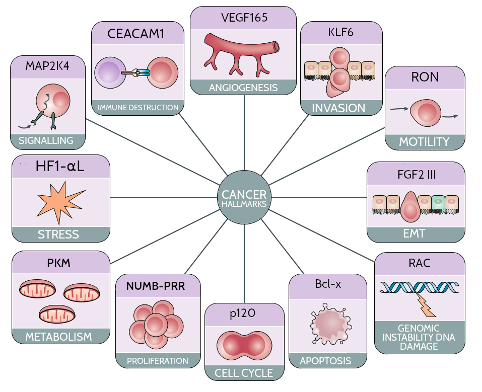 Open image in new tab
Open image in new tab
Open image in new tab
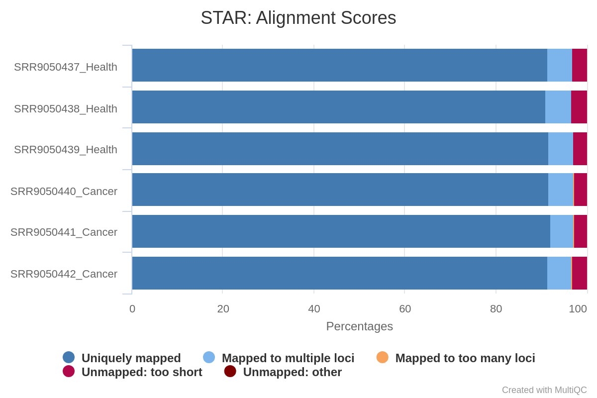 Open image in new tab
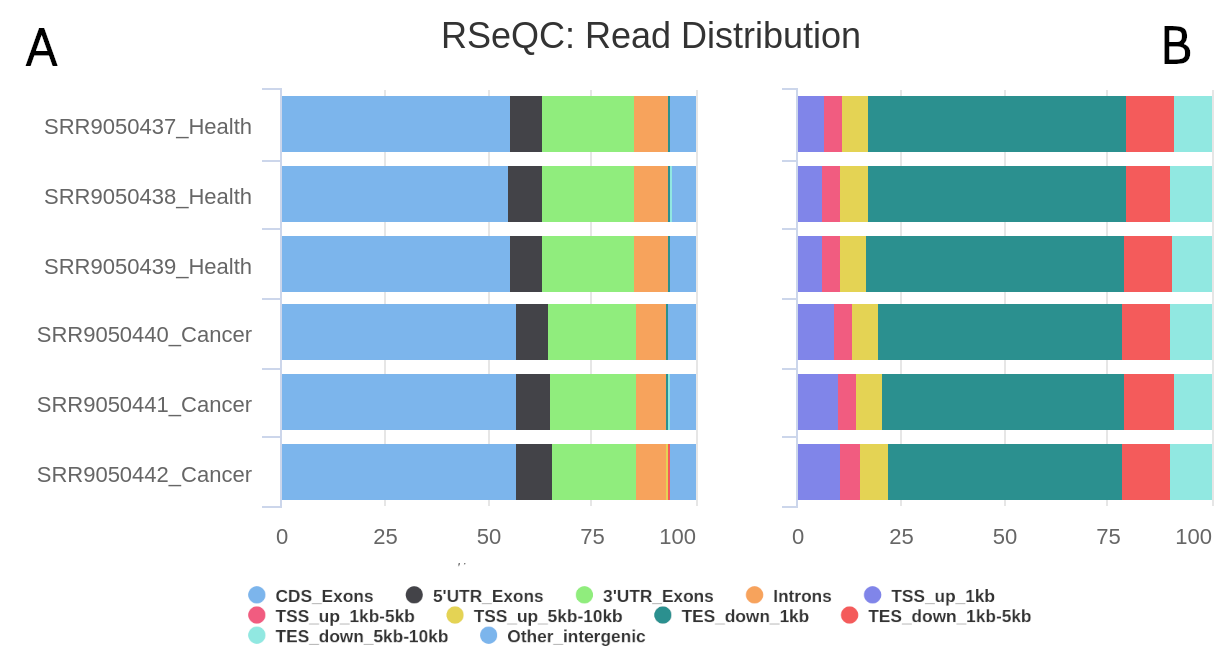 Open image in new tab
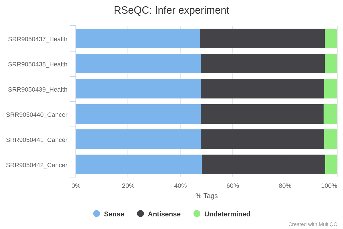 Open image in new tab
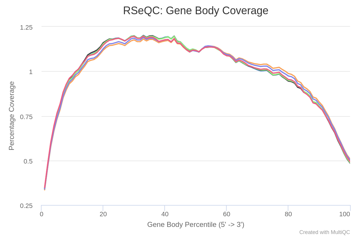 Open image in new tab
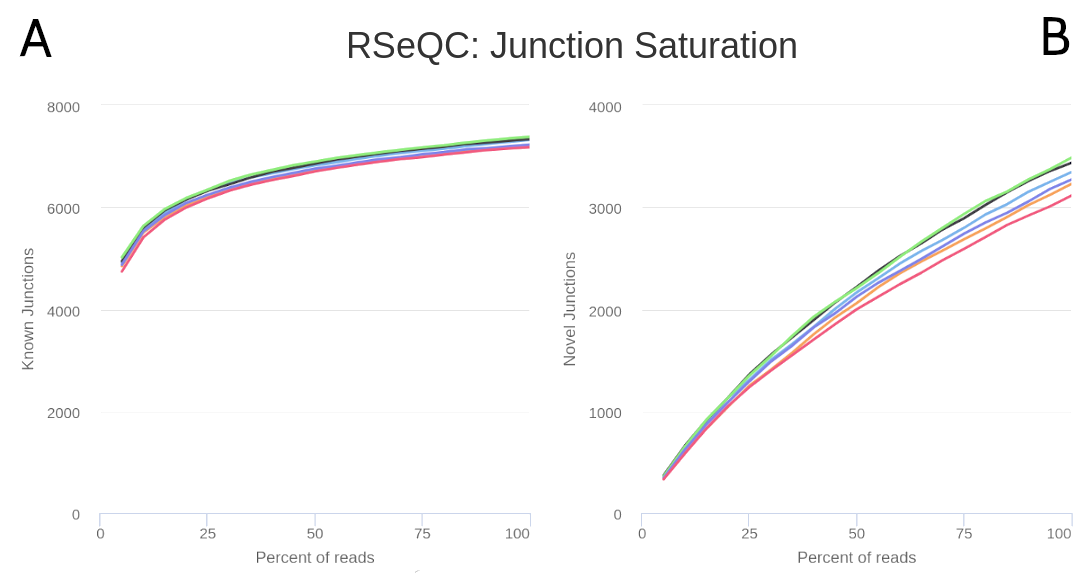 Open image in new tab
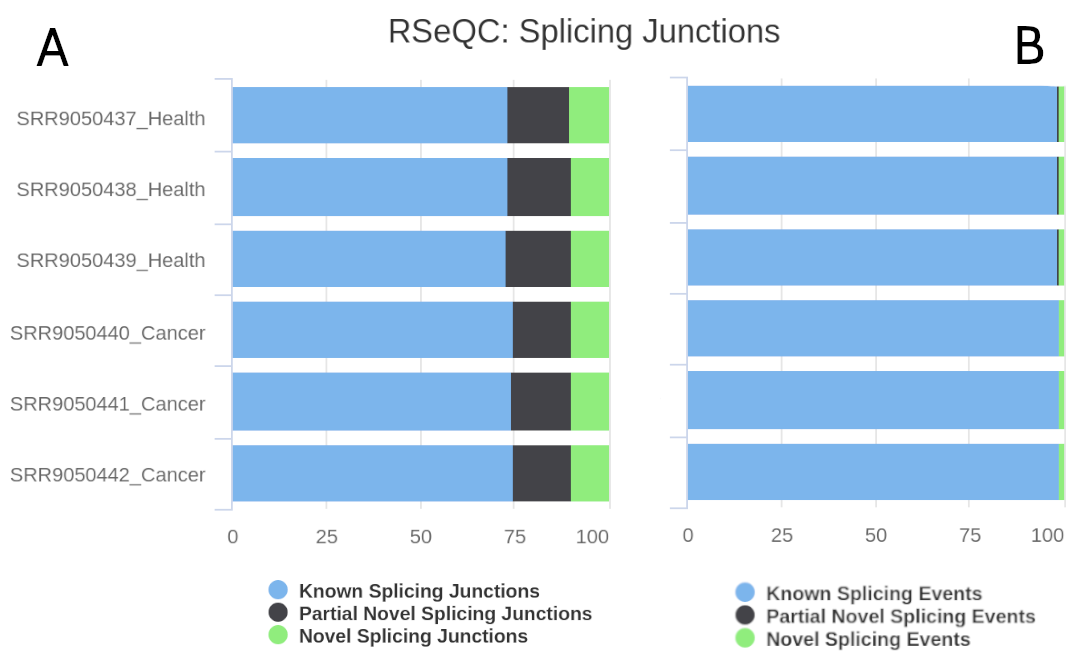 Open image in new tab
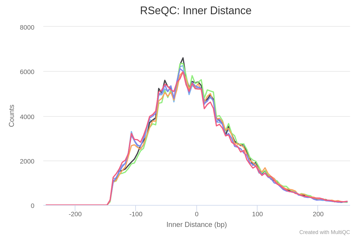 Open image in new tab
Open image in new tab
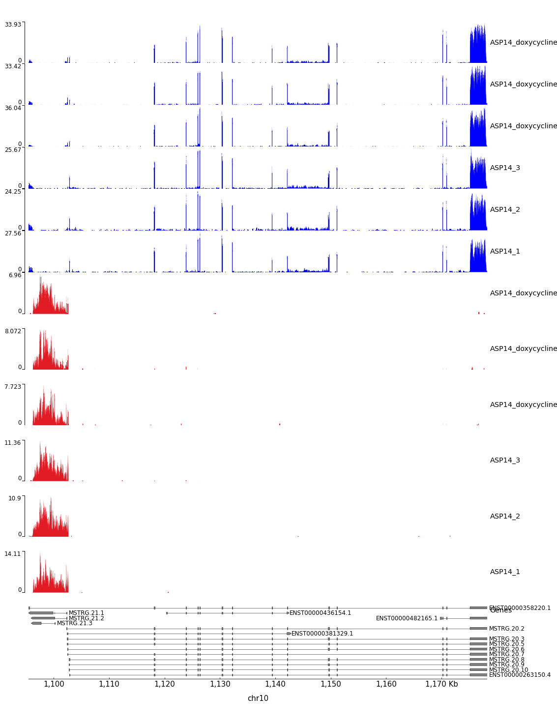 Open image in new tab
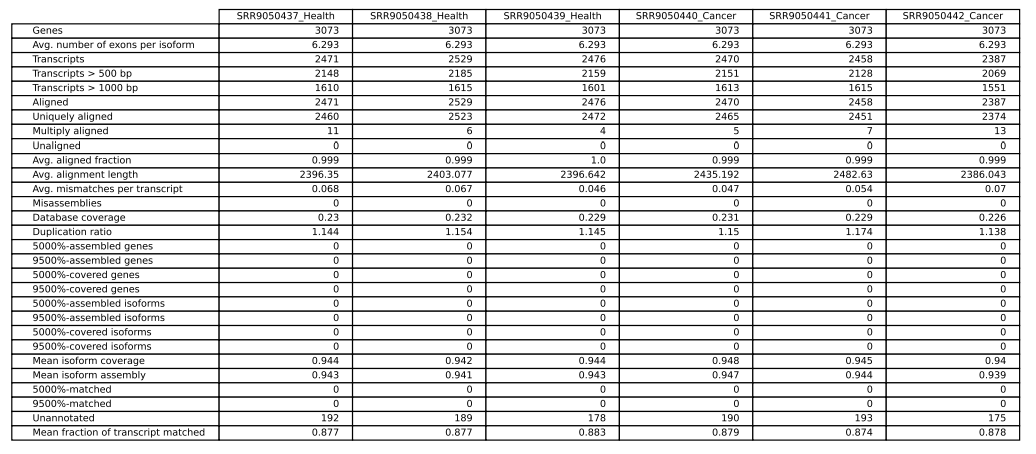 Open image in new tab
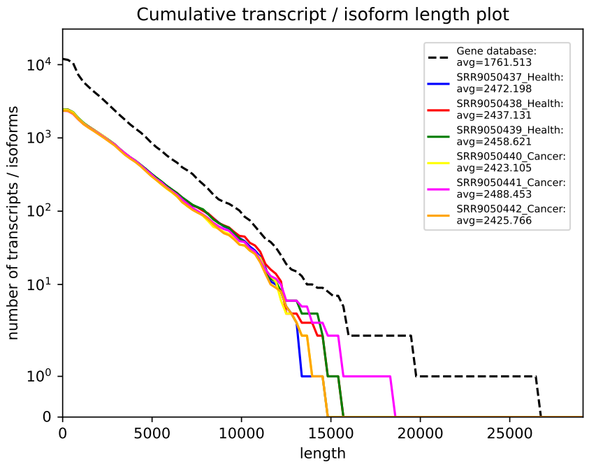 Open image in new tab
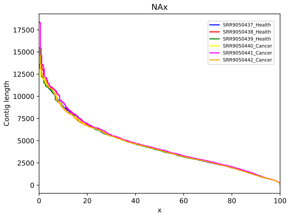 Open image in new tab
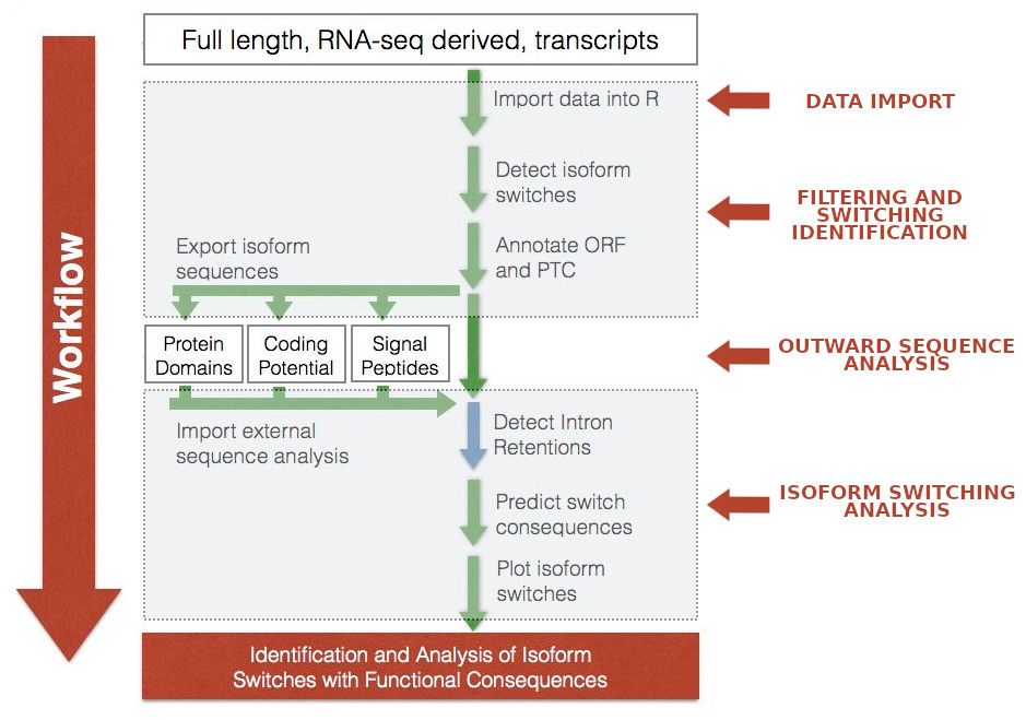 Open image in new tab
Open image in new tab
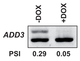 Open image in new tab
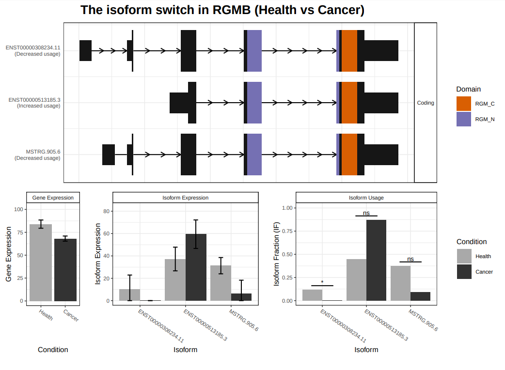 Open image in new tab
Open image in new tab
Open image in new tab
Open image in new tab
Open image in new tab
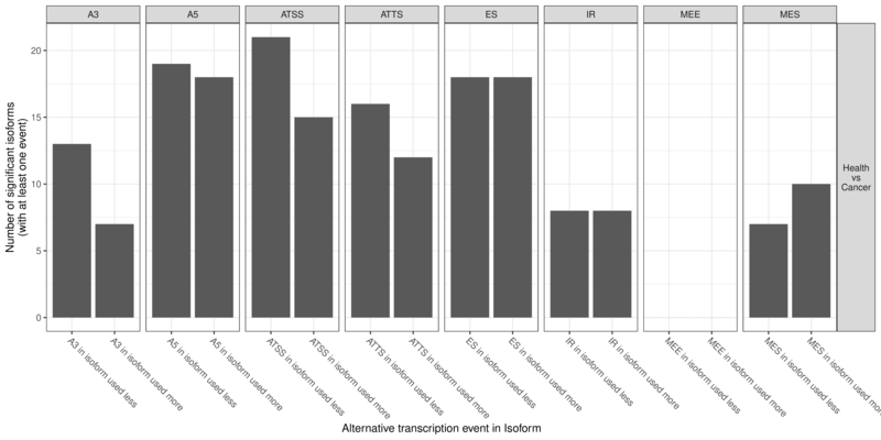 Open image in new tab
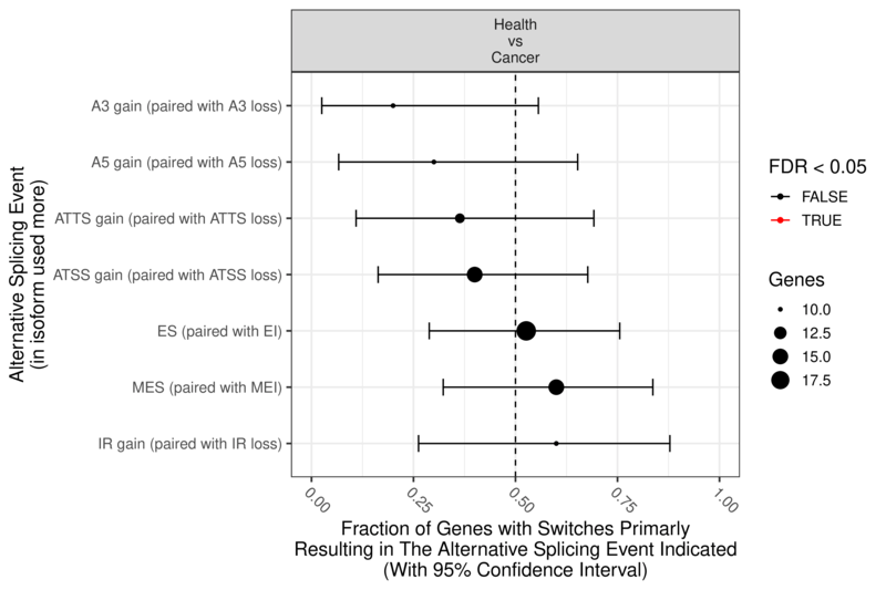 Open image in new tab
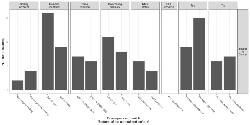 Open image in new tab
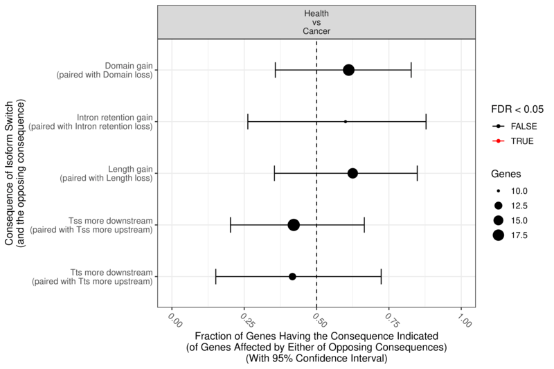 Open image in new tab
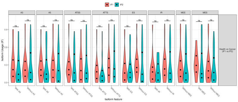 Open image in new tab
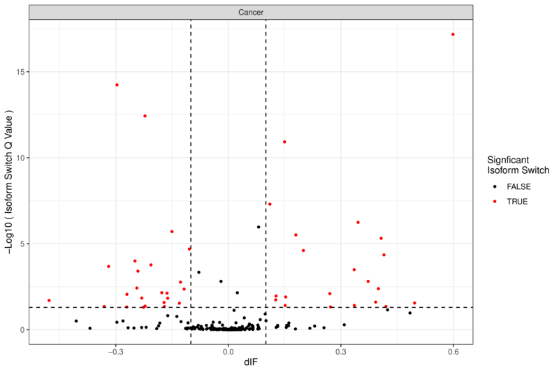 Open image in new tab
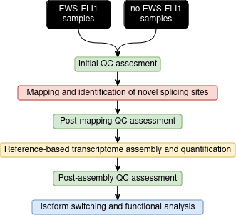 Open image in new tab