Mass spectrometry: GC-MS data processing (with XCMS, RAMClustR, RIAssigner, and matchms)
| Author(s) |
|
| Editor(s) |
|
| Reviewers |
|
OverviewQuestions:
Objectives:
What are the main steps of gas chromatography-mass spectrometry (GC-MS) data processing for metabolomic analysis?
What similarity metrics can be used to compare a pair of mass spectra and what are the differences between them?
Do you know any alternative tools that can be used in place of the individual steps of this workflow?
Requirements:
To learn about the key steps in the preprocessing and analysis of untargeted GC-MS metabolomics data.
To explore what open-source alternative tools can be used in the analysis of GC-MS data, learn about their possible parametrisations.
To analyse authentic data samples and compare them with a data library of human metabolome, composed from a collection of mostly endogenous compounds.
- Introduction to Galaxy Analyses
- slides Slides: Mass spectrometry: LC-MS preprocessing with XCMS
- tutorial Hands-on: Mass spectrometry: LC-MS preprocessing with XCMS
Time estimation: 2 hoursLevel: Intermediate IntermediateSupporting Materials:Published: May 8, 2023Last modification: Nov 9, 2023License: Tutorial Content is licensed under Creative Commons Attribution 4.0 International License. The GTN Framework is licensed under MITpurl PURL: https://gxy.io/GTN:T00344rating Rating: 5.0 (0 recent ratings, 1 all time)version Revision: 5
The study of metabolites in biological samples is routinely defined as metabolomics. Metabolomics’ studies based on untargeted mass spectrometry provide the capability to investigate metabolism on a global and relatively unbiased scale in comparison to traditional targeted studies focused on specific pathways of metabolism and a small number of metabolites. The untargeted approach enables the detection of thousands of metabolites in hypothesis-generating studies and links previously unknown metabolites with biologically important roles Patti et al. 2012. There are two major issues in contemporary mass spectrometry-based metabolomics: the first is enormous loads of signal generated during the experiments, and the second is the fact that some metabolites in the studied samples may not be known to us. These obstacles make the task of processing and interpreting the metabolomics data a cumbersome and time-consuming process Nash and Dunn 2019.
Many packages are available for the analysis of GC-MS or LC-MS data - for more details see the reviews by Stanstrup et al. 2019 and Misra 2021. In this tutorial, we focus on open-source solutions integrated within the Galaxy framework, namely XCMS, RAMClustR, RIAssigner, and matchms. In this tutorial, we will learn how to (1) extract features from the raw data using XCMS (Smith et al. 2006), (2) deconvolute the detected features into spectra with RAMClustR (Broeckling et al. 2014), (3) compute retention indices with RIAssigner (Hecht et al. 2022), and (4) identify the present compounds leveraging spectra and retention indices using matchms (Huber et al. 2020). For demonstration, we use three GC-[EI+] high-resolution mass spectrometry data files generated from quality control seminal plasma samples.
The seminal plasma samples were analyzed according to the standard operating procedure (SOP) for metabolite profiling of seminal plasma via GC Orbitrap. The 3 samples used in this training are pooled quality control (QC) samples coming from about 200 samples. The pooled samples were analyzed in dilution series to test the system suitability and the quality of the assay.
To process the data, we use several tools. XCMS (Smith et al. 2006) is a general package for untargeted metabolomics profiling. It can be used for any type of mass spectrometry acquisition (centroid and profile) or resolution (from low to high resolution), including FT-MS data coupled with a different kind of chromatography (liquid or gas). We use it to detect chromatographic peaks within our samples. Once we have detected them, they need to be deconvoluted into spectra representing chemical compounds. For that, we use RAMClustR (Broeckling et al. 2014) tool. To normalise the retention time of deconvoluted spectra in our sample, we compute the retention index using RIAssigner (Hecht et al. 2022) by comparing the data to a well-defined list of reference compound (commonly alkanes) analyzed on the same GC column. Finally, we identify detected spectra by aligning them with a database of known compounds. This can be achieved using matchms (Huber et al. 2020), resulting in a table of identified compounds weighted by a matching score.
AgendaIn this tutorial, we will cover:
Data preparation and prepocessing
Before we can start with the actual analysis pipeline, we first need to download and prepare our dataset. Many of the preprocessing steps can be run in parallel on individual samples. Therefore, we recommend using the Dataset collections in Galaxy. This can be achieved by using the dataset collection option from the beginning of your analysis when uploading your data into Galaxy.
Import the data into Galaxy
Hands On: Upload data
Create a new history for this tutorial
To create a new history simply click the new-history icon at the top of the history panel:
Import the files from Zenodo into a collection:
https://zenodo.org/record/7890956/files/8_qc_no_dil_milliq.raw
https://zenodo.org/record/7890956/files/21_qc_no_dil_milliq.raw
https://zenodo.org/record/7890956/files/29_qc_no_dil_milliq.raw
- Copy the link location
Click galaxy-upload Upload at the top of the activity panel
Click on Collection on the top
- Select galaxy-wf-edit Paste/Fetch Data
Paste the link(s) into the text field
Change Type (set all): from “Auto-detect” to
mzmlPress Start
Click on Build when available
Enter a name for the collection
- input
- Click on Create list (and wait a bit)
Make sure your data is in a collection. You can always manually create the collection from separate files:
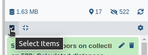
- Click on galaxy-selector Select Items at the top of the history panel
- Check all the datasets in your history you would like to include
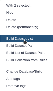
Click n of N selected and choose Advanced Build List
You are in collection building wizard. Choose Flat List and click ‘Next’ button at the right bottom corner.
Double clcik on the file names to edit. For example, remove file extensions or common prefix/suffixes to cleanup the names.
- Enter a name for your collection
- Click Build to build your collection
- Click on the checkmark icon at the top of your history again
In the further steps, this dataset collection will be referred to as
input(and we recommend naming this collection like that to avoid confusion).Import the following extra files from Zenodo:
https://zenodo.org/record/7890956/files/reference_alkanes.csv
https://zenodo.org/record/7890956/files/reference_spectral_library.msp
https://zenodo.org/record/7890956/files/sample_metadata.tsv
- Copy the link location
Click galaxy-upload Upload at the top of the activity panel
- Select galaxy-wf-edit Paste/Fetch Data
Paste the link(s) into the text field
Press Start
- Close the window
As an alternative to uploading the data from a URL or your computer, the files may also have been made available from a shared data library:
- Go into Libraries (left panel)
- Navigate to the correct folder as indicated by your instructor.
- On most Galaxies tutorial data will be provided in a folder named GTN - Material –> Topic Name -> Tutorial Name.
- Select the desired files
- Click on Add to History galaxy-dropdown near the top and select as Datasets from the dropdown menu
In the pop-up window, choose
- “Select history”: the history you want to import the data to (or create a new one)
- Click on Import
Please pay attention to the format of all uploaded files, and make sure they were correctly imported.
- Allow Galaxy to detect the datatype during Upload, and adjust from there if needed.
- Tool forms will filter for the appropriate datatypes it can use for each input.
- Directly changing a datatype can lead to errors. Be intentional and consider converting instead when possible.
- Dataset content can also be adjusted (tools: Data manipulation) and the expected datatype detected. Detected datatypes are the most reliable in most cases.
- If a tool does not accept a dataset as valid input, it is not in the correct format with the correct datatype.
- Once a dataset’s content matches the datatype, and that dataset is repeatedly used (example: Reference annotation) use that same dataset for all steps in an analysis or expect problems. This may mean rerunning prior tools if you need to make a correction.
- Tip: Not sure what datatypes a tool is expecting for an input?
- Create a new empty history
- Click on a tool from the tool panel
- The tool form will list the accepted datatypes per input
- Warning: In some cases, tools will transform a dataset to a new datatype at runtime for you.
- This is generally helpful, and best reserved for smaller datasets.
- Why? This can also unexpectedly create hidden datasets that are near duplicates of your original data, only in a different format.
- For large data, that can quickly consume working space (quota).
- Deleting/purging any hidden datasets can lead to errors if you are still using the original datasets as an input.
- Consider converting to the expected datatype yourself when data is large.
- Then test the tool directly on converted data. If it works, purge the original to recover space.
Comment: The extra filesThe three additional files contain the reference alkanes, the reference spectral library, and the sample metadata. Those files are auxiliary inputs used in the data processing and contain either extra information about the samples or serve as reference data for indexing and identification.
The list of alkanes (
.tsvor.csv) with retention times and carbon number or retention index is used to compute the retention index of the deconvoluted peaks. The alkanes should be measured in the same batch as the input sample collection.The reference spectral library (
.msp) is used for the identification of spectra. It contains the recorded and annotated mass spectra of chemical standards, ideally from a similar instrument. The unknown spectra which can be detected in the sample can then be confirmed via comparison with this library. The specific library is an in-house library of metabolite standards measured at RECETOX using a GC Orbitrap.The sample metadata (
.csvor.tsv) is a table containing information about our samples. In particular, the tabular file contains for each sample its associated sample name, class (QC, blank, sample, etc.), batch number, and injection order. It is possible to add more columns to include additional details about the samples.


As a result of this step, we should have in our history a green Dataset collection with three .raw files as well as three separate files with reference alkanes, reference spectral library, and sample metadata.
Convert the raw data to mzML
Our input data are in .raw format, which is not suitable for the downstream tools in this tutorial. We use the tool msconvert ( Galaxy version 3.0.20287.2) to convert our samples to the appropriate format (.mzML in this case).
Hands On: Convert the raw data to mzML
- msconvert ( Galaxy version 3.0.20287.2) with the following parameters:
- param-collection “Input unrefined MS data”:
input(Input dataset collection)- “Do you agree to the vendor licenses?”:
Yes- “Output Type”:
mzML- In “Data Processing Filters”:
- “Apply peak picking?”:
Yes(This option will compute centroids in the m/z domain.)Comment: Centroids
msconvertwith selected parameters computes centroids in the m/z domain. MS instruments continuously sample and record signals. Therefore, a mass peak for a single ion in one spectrum consists of multiple intensities at discrete m/z values. Centroiding is the process of reducing these mass peaks to a single representative signal, the centroid. This results in much smaller file sizes without losing too much information. In the further steps, XCMS uses the centWave chromatographic peak detection algorithm, which was designed for centroided data. That is the reason we perform the centroiding prior to chromatographic peak detection in this step.
Create the XCMS object
The first part of data processing is using the XCMS tool to detect peaks in the MS signal. For that, we first need to take the .mzML files and create a format usable by the XCMS tool. MSnbase readMSData ( Galaxy version 2.16.1+galaxy0) (Gatto and Lilley 2012. Gatto et al. 2020) takes as input our files and prepares RData files for the first XCMS step.
Hands On: Create the XCMS object
- MSnbase readMSData ( Galaxy version 2.16.1+galaxy0) with the following parameters:
- param-collection “File(s) from your history containing your chromatograms”:
input.mzML(output of msconvert tool)
- Click on param-collection Dataset collection in front of the input parameter you want to supply the collection to.
- Select the collection you want to use from the list
Comment: Output - `input.raw.RData`Collection of
rdata.msnbase.rawfiles.Rdatafile that is necessary in the next step of the workflow. These serve for an internal R representation of XCMS objects needed in the further steps.
Peak detection using XCMS
The first step in the workflow is to detect the peaks in our data using XCMS. This part, however, is covered by a separate tutorial. Although the tutorial is dedicated to LC-MS data, it can also be followed for our GC-MS data. Therefore, in this section, we do not explain this part of the workflow in detail but rather refer the reader to the dedicated tutorial. Please also pay attention to the parameter values for individual Galaxy tools, as these can differ from the referred tutorial and are adjusted to our dataset.
Since this step is already covered in a separate tutorial, it is possible to skip it. Instead, you can continue with Peak deconvolution step using a preprocessed XCMS object file prepared for you.
Hands On: Upload data
Create a new history for this tutorial
To create a new history simply click the new-history icon at the top of the history panel:
Import the following files from Zenodo:
https://zenodo.org/record/7890956/files/XCMS_object.rdata.xcms.fillpeaks
- Copy the link location
Click galaxy-upload Upload at the top of the activity panel
- Select galaxy-wf-edit Paste/Fetch Data
Paste the link(s) into the text field
Press Start
- Close the window
The format of uploaded file containing XCMS object should be
rdata.xcms.fillpeaks.
- Allow Galaxy to detect the datatype during Upload, and adjust from there if needed.
- Tool forms will filter for the appropriate datatypes it can use for each input.
- Directly changing a datatype can lead to errors. Be intentional and consider converting instead when possible.
- Dataset content can also be adjusted (tools: Data manipulation) and the expected datatype detected. Detected datatypes are the most reliable in most cases.
- If a tool does not accept a dataset as valid input, it is not in the correct format with the correct datatype.
- Once a dataset’s content matches the datatype, and that dataset is repeatedly used (example: Reference annotation) use that same dataset for all steps in an analysis or expect problems. This may mean rerunning prior tools if you need to make a correction.
- Tip: Not sure what datatypes a tool is expecting for an input?
- Create a new empty history
- Click on a tool from the tool panel
- The tool form will list the accepted datatypes per input
- Warning: In some cases, tools will transform a dataset to a new datatype at runtime for you.
- This is generally helpful, and best reserved for smaller datasets.
- Why? This can also unexpectedly create hidden datasets that are near duplicates of your original data, only in a different format.
- For large data, that can quickly consume working space (quota).
- Deleting/purging any hidden datasets can lead to errors if you are still using the original datasets as an input.
- Consider converting to the expected datatype yourself when data is large.
- Then test the tool directly on converted data. If it works, purge the original to recover space.
Peak picking
The first step is to extract peaks from each of your data files independently. For this purpose, we use the centWave chromatographic peak detection algorithm implemented in xcms findChromPeaks (xcmsSet) ( Galaxy version 3.12.0+galaxy0).
Hands On: Peak pickingxcms findChromPeaks (xcmsSet) ( Galaxy version 3.12.0+galaxy0) with the following parameters:
- param-collection “RData file”:
input.raw.RData(output of MSnbase readMSData tool)- “Extraction method for peaks detection”:
CentWave - chromatographic peak detection using the centWave method
- “Max tolerated ppm m/z deviation in consecutive scans in ppm”:
3.0- “Min,Max peak width in seconds”:
1,30- In “Advanced Options”:
- “Prefilter step for for the first analysis step (ROI detection)”:
3,500- “Noise filter”:
1000You can leave the other parameters with their default values.
Determining shared ions
At this step, you obtain a dataset collection containing one RData file per sample, with independent lists of ions. Next, we want to identify the ions shared between samples. To do so, first, you need to group your individual RData files into a single one.
Hands On: Merging filesxcms findChromPeaks Merger ( Galaxy version 3.12.0+galaxy0) with the following parameters:
- param-collection “RData file”:
input.raw.xset.RData(output of xcms findChromPeaks (xcmsSet) tool)- param-file “Sample metadata file”:
sample_metadata.tsv(Input dataset)You can leave the other parameters with their default values.
Now we can proceed with the grouping and determining shared ions among samples. The aim of this step, called grouping, is to obtain a single matrix of ions’ intensities across all samples.
Hands On: Grouping peaksxcms groupChromPeaks (group) ( Galaxy version 3.12.0+galaxy0) with the following parameters:
- param-file “RData file”:
xset.merged.RData(output of xcms findChromPeaks Merger tool)- “Method to use for grouping”:
PeakDensity - peak grouping based on time dimension peak densities
- “Bandwidth”:
3.0- “Minimum fraction of samples”:
0.9- “Width of overlapping m/z slices”:
0.01You can leave the other parameters with their default values.
Retention time correction
A deviation in retention time occurs from one sample to another, especially when you inject large sequences of samples. This step aims at correcting retention time drift for each peak among samples.
Hands On: Retention time correctionxcms adjustRtime (retcor) ( Galaxy version 3.12.0+galaxy0) with the following parameters:
- param-file “RData file”:
xset.merged.groupChromPeaks.RData(output of xcms groupChromPeaks (group) tool)- “Method to use for retention time correction”:
PeakGroups - retention time correction based on aligment of features (peak groups) present in most/all samples.
- “Minimum required fraction of samples in which peaks for the peak group were identified”:
0.7You can leave the other parameters with their default values.
Second round of determining shared ions
By applying retention time correction, the used retention time values were modified. Consequently, applying this step to your data requires completing it with an additional grouping step.
Hands On: Grouping peaksxcms groupChromPeaks (group) ( Galaxy version 3.12.0+galaxy0) with the following parameters:
- param-file “RData file”:
xset.merged.groupChromPeaks.adjustRtime.RData(output of xcms adjustRtime (retcor) tool)- “Method to use for grouping”:
PeakDensity - peak grouping based on time dimension peak densities
- “Bandwidth”:
3.0- “Minimum fraction of samples”:
0.9- “Width of overlapping m/z slices”:
0.01- “Get the Peak List”:
Yes
- “Convert retention time (seconds) into minutes”:
Yes- “If NA values remain, replace them by 0 in the dataMatrix”:
NoYou can leave the other parameters with their default values.
Integrating areas of missing peaks
At this point, the peak list may contain NA values when peaks were not considered in only some of the samples in the first peak-picking step. In this step, we will integrate the signal in the m/z-rt area of an ion (chromatographic peak group) for samples in which no chromatographic peak for this ion was identified.
Hands On: Integrating areas of missing peaksxcms fillChromPeaks (fillPeaks) ( Galaxy version 3.12.0+galaxy0) with the following parameters:
- param-file “RData file”:
xset.merged.groupChromPeaks.adjustRtime.groupChromPeaks.RData(output of xcms groupChromPeaks (group) tool)- In “Peak List”:
- “Convert retention time (seconds) into minutes”:
YesYou can leave the other parameters with their default values.
Comment: OutputAfter the
fillChromPeaksstep, you obtain your final intensity table. At this step, you have everything mandatory to begin analysing your data:
- A sampleMetadata file (if not done yet, to be completed with information about your samples)
- A dataMatrix file (with the intensities)
- A variableMetadata file (with information about ions such as retention times, m/z)
Peak deconvolution
The next step is deconvoluting the detected peaks in order to reconstruct the full spectra of the chemical compounds present in the sample, separated by the chromatography and ionized in the mass spectrometer. RAMClustR ( Galaxy version 1.3.0+galaxy0) is used to group features based on correlations across samples in a hierarchy, focusing on consistency across samples. While each feature is typically derived from a single compound and represents a fragment, the whole mass spectrum can be used to more accurately identify the precursor compound or molecular ion. RAMClustR uses a novel grouping method that operates in an unsupervised manner to group peaks into spectra without relying on the predicting in-source phenomena (in-source fragments or adduct formation) or fragmentation mechanisms.
The RAMclust similarity scoring utilises a Gaussian function, allowing flexibility in tuning correlational and retention time similarity decay rates independently, based on the dataset and the acquisition instrumentation. The correlational relationship between two features can be described by either MS-MS, MS-idMS/MS, or idMS/MS-idMS/MS values, and we support several correlation methods (e.g. Pearson’s method) to calculate similarity. These are parametrised by
sigma_tandsigma_r, Gaussian tuning parameters of retention time similarity and correlational score, respectively, between feature pairs.Similarities are then converted to dissimilarities for clustering. The similarity matrix is then clustered using one of the available methods, such as average or complete linkage hierarchical clustering. The dendrogram is cut using the
cutreeDynamicTreefunction from the packagedynamicTreeCut. For this application, the minimum module size is set to 2, dictating that only clusters with two or more features are returned, as singletons are impossible to interpret intelligently.Cluster membership, in conjunction with the abundance values from individual features in the input data, is used to create spectra. The mass to charge ratio is derived from the feature m/z, and the abundance for each m/z in the spectrum is derived from the weighted mean of the intensity values for that feature. These spectra are then exported as an
.mspformatted file, which can be directly imported by NIST MSsearch, or used as input for MassBank or NIST msPepSearch batch searching.
Hands On: Peak deconvolution
- RAMClustR ( Galaxy version 1.3.0+galaxy0) with the following parameters:
- “Choose input format:”:
XCMS
- In “Input MS Data as XCMS”:
- param-file “Input XCMS”:
xset.merged.groupChromPeaks.adjustRtime.groupChromPeaks.fillChromPeaks.RData(output of xcms fillChromPeaks (fillPeaks) tool)- In “General parameters”:
- “Sigma r”:
0.7- “Maximum RT difference”:
10.0- In “Clustering”:
- “Minimal cluster size”:
5- “Maximal tree height”:
0.9You can leave the other parameters with their default values.
The spectral data comes as an .msp file, which is a text file structured according to the NIST MSSearch spectra format. .msp is one of the generally accepted formats for mass spectral libraries (or collections of unidentified spectra, so called spectral archives), and it is compatible with lots of spectra processing programmes (MS-DIAL, NIST MS Search, AMDIS, etc.). Because .msp files are text-based, they can be viewed as simple txt files:
Hands On: Data ExplorationClick “View data” galaxy-eye icon next to the dataset in the Galaxy history. The contents of the file would look like this:
Dataset icons and their usage:
- galaxy-eye “Eye icon”: Display dataset contents.
- galaxy-pencil “Pencil icon”: Edit attributes of dataset metadata: labels, datatype, database.
- galaxy-delete “Trash icon”: Delete the dataset.
- galaxy-save “Disc icon”: Download the dataset.
- galaxy-link “Copy link”: Copy link URL to the dataset.
- galaxy-info “Info icon”: Dataset details and job runtime information: inputs, parameters, logs.
- galaxy-refresh “Refresh/Rerun icon”: Run this (selected) job again or examine original submitted form.
- galaxy-barchart “Visualize icon”: External display links (UCSC, IGV, NPL, PV); Charts and graphing; Editor (manually edit text).
- galaxy-dataset-map “Dataset Map icon”: Filter the history for related Input/Output Datasets. Click again to clear the filter.
- galaxy-bug “Bug icon”: Review subset of logs (review all under galaxy-info), and optionally submit a bug report.
NAME:C001 IONMODE:Negative SPECTRUMTYPE:Centroid RETENTIONTIME:383.27 Num Peaks:231 217.1073 64041926 243.0865 35597866 257.1134 31831229 224.061 27258239 258.11 24996353 241.0821 23957171 315.1188 13756744 ... NAME:C002 IONMODE:Negative SPECTRUMTYPE:Centroid RETENTIONTIME:281.62 Num Peaks:165 307.1573 299174880 147.0654 298860831 149.0447 287809889 218.1066 118274758 189.076 112486871 364.1787 75134143 191.0916 52526567 308.1579 52057158 ...You might wonder how can the ionisation mode (IONMODE) for GC-MS data be negative when using electron impact (EI+) ionization. This is, of course, incorrect. This is actually just a default behaviour of RAMClustR. We can optionally change this by providing RAMClustR an experiment definition file. This file can be created manually or using the RAMClustR define experiment ( Galaxy version 1.0.2) tool. There we can specify annotations such as what instrument we used or ionisation mode (which was EI+ in our case), and this will be transfered to the
.mspfile. Finally, we can provide such a file as an input to RAMClustR in the Extras inputs section.
.msp files can contain one or more mass spectra, these are split by an empty line. The individual spectra essentially consist of two sections: metadata and peaks. The metadata consists of compound name, spectrum type (which is centroid in this case), ion mode, retention time, and the number of m/z peaks. If the compound has not been identified, as in our case, the NAME can be any arbitrary string. It is best, however, if that string is unique within that .msp file. The metadata fields are usually unordered, so it is quite common for one .msp file to contain NAME as the first metadata key and for another .msp to have this key somewhere in the middle. The keys themselves also aren’t strictly defined and can have different names (e.g., compound_name instead of NAME). The msp format is inherently not standardized and various flavours exist.
However, as we can observe, the metadata part is rather incomplete. We would like to gather more information about the detected spectra and identify the specific compounds corresponding to them.
The second output file is the so called Spec Abundance table, containing the expression of all deconvoluted spectra across all samples. It is the corresponding element to the peak intensity table obtained from XCMS, only for the whole deconvoluted spectrum. This file is used for further downstream processing and analysis of the data and eventual comparisons across different sample types or groups. For more information on this downstream data processing see this tutorial.
Retention index calculation
The retention index (Van Den Dool and Kratz 1963) is a way how to convert equipment- and experiment-specific retention times into system-independent normalised constants for GC-based experiments. The retention index of a compound is computed from the retention time by interpolating between the retention times adjacent alkanes which are assigned a fixed retention index. This can be different for the individual chromatographic system, but the derived retention indices are independent and allow comparing values measured by different analytical laboratories.
We use the package RIAssigner ( Galaxy version 0.3.4+galaxy1) to compute retention indices for files in the .msp format using an indexed reference list of alkanes in .csv or .msp format. The output follows the same format as the input but with added retention index values. These can be used at a subsequent stage to improve compound identification (Kumari et al. 2011). Multiple computation methods (e.g. piecewise-linear or cubic spline) are supported by the tool.
Hands On: Retention index calculation
- RIAssigner ( Galaxy version 0.3.4+galaxy1) with the following parameters:
- In “Query dataset”:
- param-file “Query compound list”:
Mass spectra from RAMClustR(output of RAMClustR tool)- In “Reference dataset”:
- param-file “Reference compound list”:
reference_alkanes.csv(Input dataset)You can leave the other parameters with their default values.
Comment: Minutes vs. secondsYou might notice that in the last XCMS step, we converted the retention times to minutes. However, in this step, we are using seconds again. The reason is that RAMClustR converted them internally again to seconds. Regarding the reference compound list, this database already has its retention times in seconds.
The Kováts retention index (or Kováts index) of a compound is its retention time normalized to the retention times of adjacently eluting n-alkanes. It is based on the fact that the logarithm of the retention time converges to the number of carbon atoms in the alkane. For an isothermal chromatogram, you use the following equation to calculate the Kováts index:
\[I = 100 \times \frac{\mathtt{log}~t\_x - \mathtt{log}~t\_n}{\mathtt{log}~t\_{n+1} - \mathtt{log}~t\_n}\]where \(t\_n\) and \(t\_{n+1}\) are retention times of the reference n-alkane hydrocarbons eluting immediately before and after chemical compound X and \(t\_x\) is the retention time of compound X.
In practice, first, you run a chromatogram of a standard alkane mixture in the range of interest. Then you do a co-injection of your sample with the standard alkanes. The main advantage of this method is reproducibility.
Identification
To annotate and putatively identify the deconvoluted spectra, we compare them with a reference spectral library. This library contains spectra of standards measured on the same instrument for optimal comparability. The matchms package is used for spectral matching. It was built to import and apply different similarity measures to compare large numbers of spectra. This includes common cosine scores but can also easily be extended with custom similarity measures. For more information on how to use matchms from Python check out this blog.
Fragmentation patterns of ions (spectra) are widely used in the process of compound identification for EI+ ionization in complex mixtures. The number of identifiable compounds and associated data keeps growing with the increasing sensitivity and resolution of mass spectrometers. These data are clustered into collections of chemical structures and their spectra, also called spectral libraries (Stein 1995, Stein 2012), which can be used for fast, reliable identifications for any compound whose fragmentation pattern is measured by the instrument.
To identify the compounds after GC/MS analysis, the library searching is performed for every detected spectrum. This locates the most similar spectra in the reference library, providing a list of the potential identifications sorted by computed similarity. Indeed, a library search should also yield the confidence of compound identification, often expressed as a similarity score.
Reference libraries’ users usually expect their reliability to be quite high. However, there are many sources of error which we need to be aware of. A particularly error-prone aspect is annotation. Even an excellent spectrum becomes worthless for a wrongly annotated compound. A variety of computer-aided quality control measures can help to improve these issues, but libraries always require some level of expert human decision-making before a spectrum is added to the library. This is also important for redundant and unidentified spectra.
Compute similarity scores
We use the cosine score with a greedy peak pairing heuristic to compute the number of matching ions with a given tolerance and the cosine scores for the matched peaks. Compared to more traditional methods of forward and reverse matching, matchms is performing matching on peaks present both in the measured sample and the reference data. This inherently yields higher scores than the forward and reverse scoring used by NIST.
One of the most common methods to compute the similarity score between two spectra is computing the cosine of the angle between them. Each spectrum can be represented as a vector with an axis along each of its m/z values. Then the cosine of the angle is basically a normalised dot product of these two vectors. The intensity and m/z weighting corrections have been used to optimise performance. For example, higher mass peaks can be given greater weight since they are more discriminating than lower mass peaks. Reverse scores assign no weight to peaks present only in the measured sample spectrum under the assumption that they arise from impurities.
Hands On: Compute similarity scores
- matchms similarity ( Galaxy version 0.20.0+galaxy0) with the following parameters:
- param-file “Queries spectra”:
RI using kovats of Mass spectra from RAMClustR(output of RIAssigner tool)- “Symmetric”:
No(if we were to query our spectra agains itself, we would selectYes)
- param-file “Reference spectra”:
reference_spectral_library.msp(downloaded file from Zenodo)- In “Algorithm Parameters”:
- “tolerance”:
0.03- “Apply RI filtering”:
Yes(we use this since our data is GC)You can leave the other parameters with their default values.
Comment: Used reference spectraThe RECETOX Metabolome HR-[EI+]-MS library is a collection of mostly endogenous compounds from the MetaSci Human Metabolite Library. Analytes underwent methoximation/silylation prior to acquisition. Spectra were acquired at 70 eV on Thermo Fisher Q Exactive™ GC Orbitrap™ GC-MS/MS at 60000 resolving power.
Cosine Greedy
The cosine score, also known as the dot product, is based on representing the similarity of two spectra through the cosine of an angle between the vectors that the spectra produce. Two peaks are considered as matching if their m/z values lie within the given tolerance. Cosine greedy looks up matching peaks in a “greedy” way, which does not always lead to the most optimal alignments.
This score was among the first to be used for looking up matching spectra in spectral libraries and, to this day, remains one of the most popular scoring methods for both library matching and molecular networking workflows.
Cosine Hungarian
This method computes the similarities in the same way as the Cosine Greedy but with a difference in m/z peak alignment. The difference lies in that the Hungarian algorithm is used here to find matching peaks. This leads to the best peak pairs match but can take significantly longer than the “greedy” algorithm.
Modified Cosine
Modified Cosine is another, as its name states, representative of the family of cosine-based scores. This method aligns peaks by finding the best possible matches and considers two peaks a match if their m/z values are within tolerance before or after a mass-shift is applied. A mass shift is essentially a difference of precursor-m/z of two compared spectra. The similarity is then again expressed as a cosine of the angle between two vectors.
Neutral Losses Cosine
Neutral Loss metric works similarly to all described above with one major difference: instead of encoding the spectra as “intensity vs m/z” vector, it encodes it to an “intensity vs Δm/z”, where delta is computed as an m/z difference between precursor and a fragment m/z. This, in theory, could better capture the underlying structural similarities between molecules.
Format the output
The output of the previous step is a json file. This format is very simple to read for our computers, but not so much for us. We can use the matchms scores formatter ( Galaxy version 0.20.0+galaxy0) to convert the data to a tab-separated file with a scores matrix.
The output table contains the scores and number of matched ions of the deconvoluted spectra with the spectra in the reference library. The raw output can be filtered to only contain the top matches (3 by default) and/or to contain only pairs with a score and number of matched ions larger than provided thresholds.
Hands On: Format the output
- matchms scores formatter ( Galaxy version 0.20.0+galaxy0) with the following parameters:
- param-file “Scores object”:
CosineGreedy scores(output of matchms similarity tool)You can leave the other parameters with their default values.
query reference CosineGreedy_score CosineGreedy_matches C044 Guanine_3TMS 0.987 19 C068 Tryptophan_3TMS 0.981 9 C053 Norleucine_2TMS 0.980 12 … … … …
At this stage, all steps are complete: we have the list of identified spectra corresponding to a compound from the reference database. Since this process is dependent on the parameters we used along the way, the result should be considered dependent on them. To enumerate this dependency, each potential compound has been assigned a confidence score.
Conclusion
In this tutorial, we show how untargeted GC-MS data can be processed to obtain tentative identification of compounds contained in the analyzed samples. Using XCMS, we obtain a peak and intensity table from our files which contains information about the detected ions (such as m/z and retention time) and their intensities across all samples. Afterwards, we used RAMClustR to reconstruct the fragmentation spectra which we assume to originate from the analyzed compounds contained within our samples. We use a correlation based approach which allows us to reconstruct also low-abundant features as long as their intensities are correlating across samples. This method is different than the sample-wise deconvolution using CAMERA (Kuhl et al. 2012). To have more information available for compound identification, we computed the retention index using RIAssigner and added it to our deconvoluted spectra. We then finally compare the deconvoluted spectra against the reference library using matchms, using a retention index threshold to pre-filter our matches and then computing the cosine similarity for the spectra within the retention index tolerance.
This workflow leverages the correlation of features across samples to improve the annotation performance, trying to capture even low abundant signals. It is suitable for both high- and low-resolution GC-MS data acquired in either profile or centroid mode by adapting the individual tool parameters or in-/excluding individual steps which are specific to a certain data format.
Before further statistical analysis, the information from the scores table can be included in the library of deconvoluted spectra manually to add the putative identifications. The further processing can then leverage this information and the intensity information contained in the SpecAbundance output from RAMclustR.
Note that this tutorial doesn’t cover all steps which are possible or compatible with this workflow. Other options include the matchms filtering ( Galaxy version 0.17.0+galaxy0) tool with which you can normalize your spectra or remove low-abundant ions before matching. Another option for normalization outside of the built-in normalization tools of RAMClustR is the WaveICA ( Galaxy version 0.2.0+galaxy2) tool for correction of batch effects.
You've Finished the Tutorial
Key points
The processing of untargeted GC-MS metabolomic data can be done using open-source tools.
This processing workflow is complementary to CAMERA and metaMS.
Frequently Asked Questions
Have questions about this tutorial? Have a look at the available FAQ pages and support channelsReferences
- Van Den Dool, H., and P. D. Kratz, 1963 A generalization of the retention index system including linear temperature programmed gas-liquid partition chromatography: 463–471 p. 10.1016/S0021-9673(01)80947-X https://www.sciencedirect.com/science/article/pii/S002196730180947X
- Stein, S. E., 1995 Chemical substructure identification by mass spectral library searching. Journal of the American Society for Mass Spectrometry 6: 644–655. 10.1016/1044-0305(95)00291-K
- Smith, C. A., E. J. Want, G. O’Maille, R. Abagyan, and G. Siuzdak, 2006 XCMS: Processing Mass Spectrometry Data for Metabolite Profiling Using Nonlinear Peak Alignment, Matching, and Identification. Analytical Chemistry 78: 779–787. 10.1021/ac051437y
- Kumari, S., D. Stevens, T. Kind, C. Denkert, and O. Fiehn, 2011 Applying in-silico retention index and mass spectra matching for identification of unknown metabolites in accurate mass GC-TOF mass spectrometry. Analytical chemistry 83: 5895–5902. 10.1021/ac2006137
- Gatto, L., and K. S. Lilley, 2012 MSnbase-an R/Bioconductor package for isobaric tagged mass spectrometry data visualization, processing and quantitation. Bioinformatics 28: 288–289. 10.1093/bioinformatics/btr645
- Kuhl, C., R. Tautenhahn, C. Böttcher, T. R. Larson, and S. Neumann, 2012 CAMERA: An Integrated Strategy for Compound Spectra Extraction and Annotation of Liquid Chromatography/Mass Spectrometry Data Sets. Analytical Chemistry 84: 283–289. 10.1021/ac202450g https://pubs.acs.org/doi/10.1021/ac202450g
- Patti, G. J., O. Yanes, and G. Siuzdak, 2012 Metabolomics: the apogee of the omics trilogy. Nature Reviews Molecular Cell Biology 13: 263–269. 10.1038/nrm3314 http://www.nature.com/articles/nrm3314
- Stein, S., 2012 Mass spectral reference libraries: an ever-expanding resource for chemical identification. 10.1021/ac301205z
- Broeckling, C. D., F. A. Afsar, S. Neumann, A. Ben-Hur, and J. E. Prenni, 2014 RAMClust: a novel feature clustering method enables spectral-matching-based annotation for metabolomics data. Analytical chemistry 86: 6812–6817. 10.1021/ac501530d
- Nash, W. J., and W. B. Dunn, 2019 From mass to metabolite in human untargeted metabolomics: Recent advances in annotation of metabolites applying liquid chromatography-mass spectrometry data. TrAC Trends in Analytical Chemistry 120: 115324. 10.1016/j.trac.2018.11.022
- Stanstrup, J., C. Broeckling, R. Helmus, N. Hoffmann, E. Mathé et al., 2019 The metaRbolomics Toolbox in Bioconductor and beyond. Metabolites 9: 200. 10.3390/metabo9100200 https://www.mdpi.com/2218-1989/9/10/200
- Gatto, L., S. Gibb, and J. Rainer, 2020 MSnbase, efficient and elegant R-based processing and visualization of raw mass spectrometry data. Journal of Proteome Research 20: 1063–1069. 10.1021/acs.jproteome.0c00313
- Huber, F., S. Verhoeven, C. Meijer, H. Spreeuw, E. M. V. Castilla et al., 2020 matchms - processing and similarity evaluation of mass spectrometry data. Journal of Open Source Software 5: 2411. 10.21105/joss.02411
- Misra, B. B., 2021 New software tools, databases, and resources in metabolomics: updates from 2020. Metabolomics 17: 49. 10.1007/s11306-021-01796-1 ISBN: 0123456789
- Hecht, H., M. Skoryk, M. Čech, and E. J. Price, 2022 RIAssigner: A package for gas chromatographic retention index calculation. Journal of Open Source Software 7: 4337. 10.21105/joss.04337
Feedback
Did you use this material as an instructor? Feel free to give us feedback on how it went.
Did you use this material as a learner or student? Click the form below to leave feedback.

Citing this Tutorial
- Matej Troják, Helge Hecht, Maxim Skoryk, Mass spectrometry: GC-MS data processing (with XCMS, RAMClustR, RIAssigner, and matchms) (Galaxy Training Materials). https://training.galaxyproject.org/training-material/topics/metabolomics/tutorials/gc_ms_with_xcms/tutorial.html Online; accessed TODAY
- Hiltemann, Saskia, Rasche, Helena et al., 2023 Galaxy Training: A Powerful Framework for Teaching! PLOS Computational Biology 10.1371/journal.pcbi.1010752
- Batut et al., 2018 Community-Driven Data Analysis Training for Biology Cell Systems 10.1016/j.cels.2018.05.012
Congratulations on successfully completing this tutorial!@misc{metabolomics-gc_ms_with_xcms, author = "Matej Troják and Helge Hecht and Maxim Skoryk", title = "Mass spectrometry: GC-MS data processing (with XCMS, RAMClustR, RIAssigner, and matchms) (Galaxy Training Materials)", year = "", month = "", day = "", url = "\url{https://training.galaxyproject.org/training-material/topics/metabolomics/tutorials/gc_ms_with_xcms/tutorial.html}", note = "[Online; accessed TODAY]" } @article{Hiltemann_2023, doi = {10.1371/journal.pcbi.1010752}, url = {https://doi.org/10.1371%2Fjournal.pcbi.1010752}, year = 2023, month = {jan}, publisher = {Public Library of Science ({PLoS})}, volume = {19}, number = {1}, pages = {e1010752}, author = {Saskia Hiltemann and Helena Rasche and Simon Gladman and Hans-Rudolf Hotz and Delphine Larivi{\`{e}}re and Daniel Blankenberg and Pratik D. Jagtap and Thomas Wollmann and Anthony Bretaudeau and Nadia Gou{\'{e}} and Timothy J. Griffin and Coline Royaux and Yvan Le Bras and Subina Mehta and Anna Syme and Frederik Coppens and Bert Droesbeke and Nicola Soranzo and Wendi Bacon and Fotis Psomopoulos and Crist{\'{o}}bal Gallardo-Alba and John Davis and Melanie Christine Föll and Matthias Fahrner and Maria A. Doyle and Beatriz Serrano-Solano and Anne Claire Fouilloux and Peter van Heusden and Wolfgang Maier and Dave Clements and Florian Heyl and Björn Grüning and B{\'{e}}r{\'{e}}nice Batut and}, editor = {Francis Ouellette}, title = {Galaxy Training: A powerful framework for teaching!}, journal = {PLoS Comput Biol} }
You can use Ephemeris's
shed-tools installcommand to install the tools used in this tutorial.shed-tools install [-g GALAXY] [-a API_KEY] -t <(curl https://training.galaxyproject.org/training-material/api/topics/metabolomics/tutorials/gc_ms_with_xcms/tutorial.json | jq .admin_install_yaml -r)Alternatively you can copy and paste the following YAML
---
install_tool_dependencies: true
install_repository_dependencies: true
install_resolver_dependencies: true
tools:
- name: msconvert
  owner: galaxyp
  revisions: 6153e8ada1ee
  tool_panel_section_label: Convert Formats
  tool_shed_url: https://toolshed.g2.bx.psu.edu/
- name: msnbase_readmsdata
  owner: lecorguille
  revisions: 11ab2081bd4a
  tool_panel_section_label: Metabolomics
  tool_shed_url: https://toolshed.g2.bx.psu.edu/
- name: xcms_fillpeaks
  owner: lecorguille
  revisions: 26d77e9ceb49
  tool_panel_section_label: Metabolomics
  tool_shed_url: https://toolshed.g2.bx.psu.edu/
- name: xcms_group
  owner: lecorguille
  revisions: d45a786cbc40
  tool_panel_section_label: Metabolomics
  tool_shed_url: https://toolshed.g2.bx.psu.edu/
- name: xcms_merge
  owner: lecorguille
  revisions: 5bd125a3f3b0
  tool_panel_section_label: Metabolomics
  tool_shed_url: https://toolshed.g2.bx.psu.edu/
- name: xcms_retcor
  owner: lecorguille
  revisions: aa252eec9229
  tool_panel_section_label: Metabolomics
  tool_shed_url: https://toolshed.g2.bx.psu.edu/
- name: xcms_xcmsset
  owner: lecorguille
  revisions: b02d1992a43a
  tool_panel_section_label: Metabolomics
  tool_shed_url: https://toolshed.g2.bx.psu.edu/
- name: matchms_filtering
  owner: recetox
  revisions: 357df6c47d92
  tool_panel_section_label: Metabolomics
  tool_shed_url: https://toolshed.g2.bx.psu.edu/
- name: matchms_formatter
  owner: recetox
  revisions: 1b09315a3f87
  tool_panel_section_label: Metabolomics
  tool_shed_url: https://toolshed.g2.bx.psu.edu/
- name: matchms_similarity
  owner: recetox
  revisions: e5010b19d64d
  tool_panel_section_label: Metabolomics
  tool_shed_url: https://toolshed.g2.bx.psu.edu/
- name: ramclustr
  owner: recetox
  revisions: 2ec9253a647e
  tool_panel_section_label: Metabolomics
  tool_shed_url: https://toolshed.g2.bx.psu.edu/
- name: ramclustr
  owner: recetox
  revisions: 050cfef6ba65
  tool_panel_section_label: Metabolomics
  tool_shed_url: https://toolshed.g2.bx.psu.edu/
- name: ramclustr_define_experiment
  owner: recetox
  revisions: 25625114618e
  tool_panel_section_label: Metabolomics
  tool_shed_url: https://toolshed.g2.bx.psu.edu/
- name: riassigner
  owner: recetox
  revisions: c702620c22b1
  tool_panel_section_label: Metabolomics
  tool_shed_url: https://toolshed.g2.bx.psu.edu/
- name: waveica
  owner: recetox
  revisions: b77023c41c76
  tool_panel_section_label: Metabolomics
  tool_shed_url: https://toolshed.g2.bx.psu.edu/