Best viewed in RStudio

This tutorial is available as an RMarkdown file and best viewed in RStudio! You can load this notebook in RStudio on one of the UseGalaxy.* servers

Launching the notebook in RStudio in Galaxy

1. Instructions to Launch RStudio
2. Access the R console in RStudio (bottom left quarter of the screen)
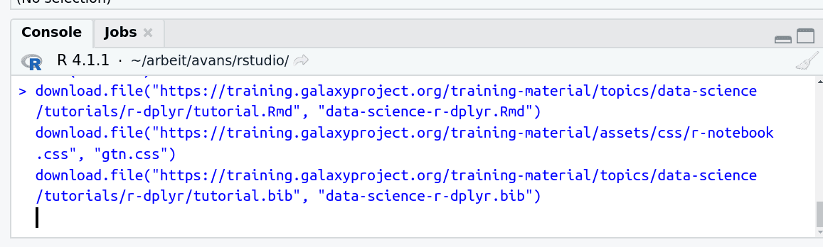
3. Run the following code:

   download.file("https://training.galaxyproject.org/training-material/topics/data-science/tutorials/sql-r/data-science-sql-r.Rmd", "data-science-sql-r.Rmd")
   download.file("https://training.galaxyproject.org/training-material/assets/css/r-notebook.css", "gtn.css")
   

4. Double click the RMarkdown document that appears in the list of files on the right.

Downloading the notebook

1. Right click this link: tutorial.Rmd
2. Save Link As...

Alternative Formats

1. This tutorial is also available as a Jupyter Notebook (With Solutions), Jupyter Notebook (Without Solutions)

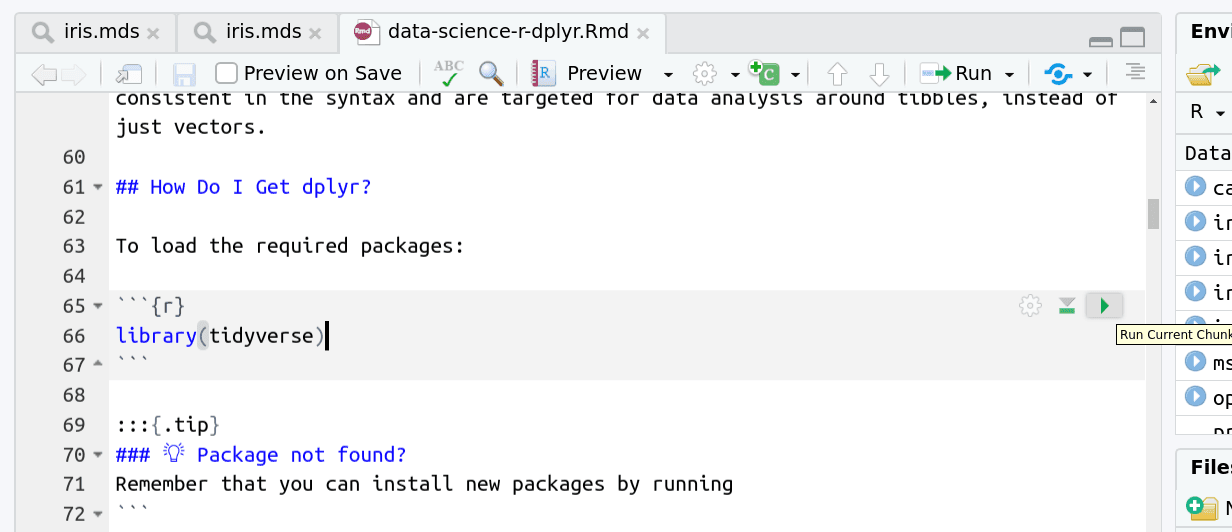
Hands-on: Learning with RMarkdown in RStudio

Learning with RMarkdown is a bit different than you might be used to. Instead of copying and pasting code from the GTN into a document you’ll instead be able to run the code directly as it was written, inside RStudio! You can now focus just on the code and reading within RStudio.

1. Load the notebook if you have not already, following the tip box at the top of the tutorial

   

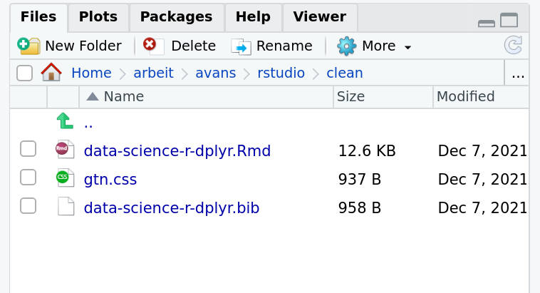
2. Open it by clicking on the .Rmd file in the file browser (bottom right)

   

3. The RMarkdown document will appear in the document viewer (top left)

   

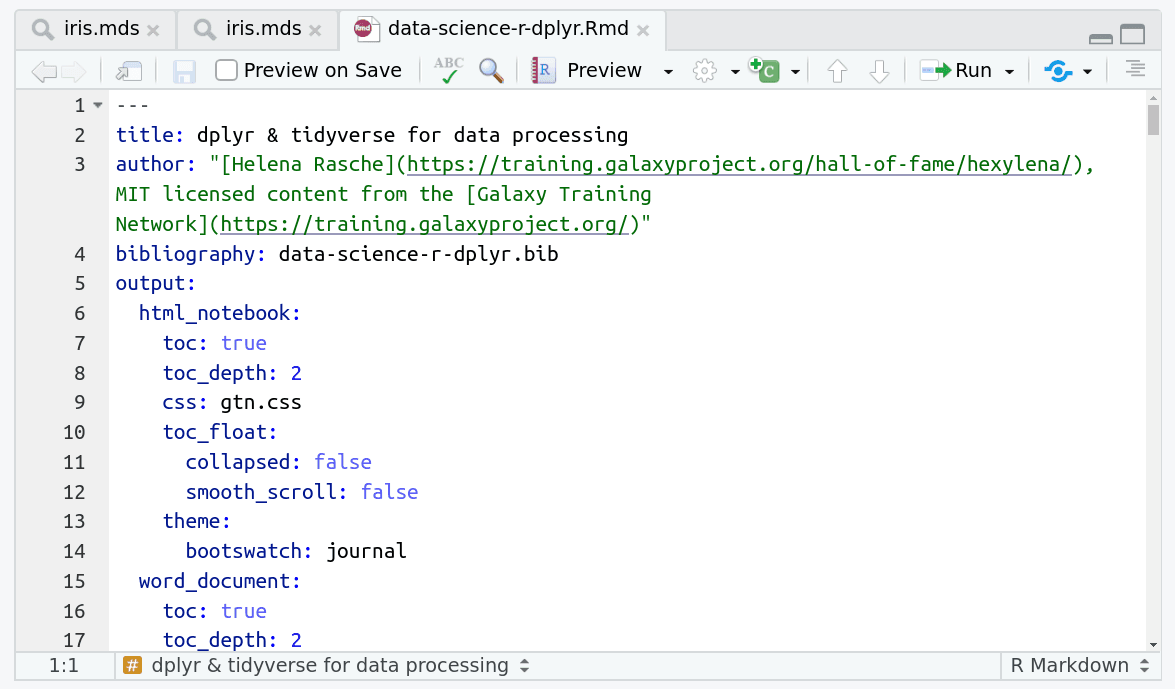
You’re now ready to view the RMarkdown notebook! Each notebook starts with a lot of metadata about how to build the notebook for viewing, but you can ignore this for now and scroll down to the content of the tutorial.

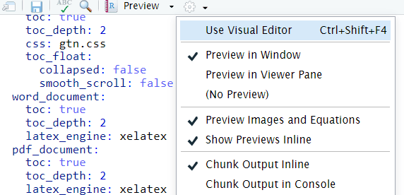
You can switch to the visual mode which is way easier to read - just click on the gear icon and select Use Visual Editor.

You’ll see codeblocks scattered throughout the text, and these are all runnable snippets that appear like this in the document:

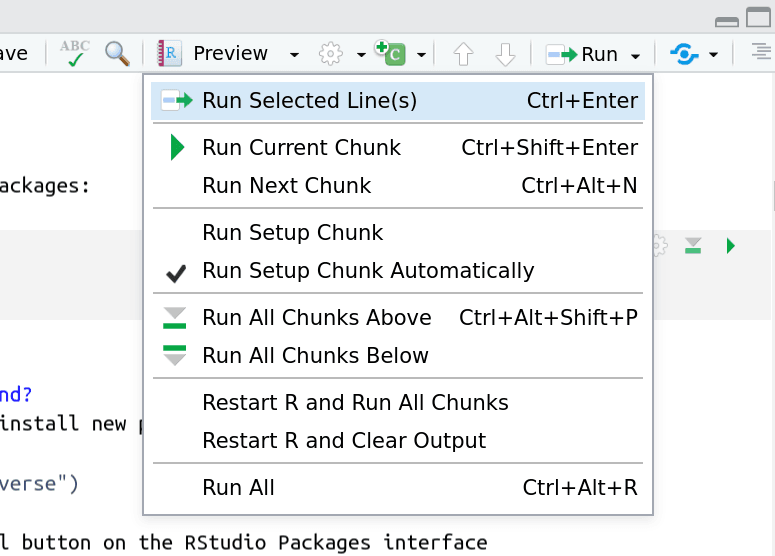
And you have a few options for how to run them:

1. Click the green arrow
2. ctrl+enter

3. Using the menu at the top to run all

   

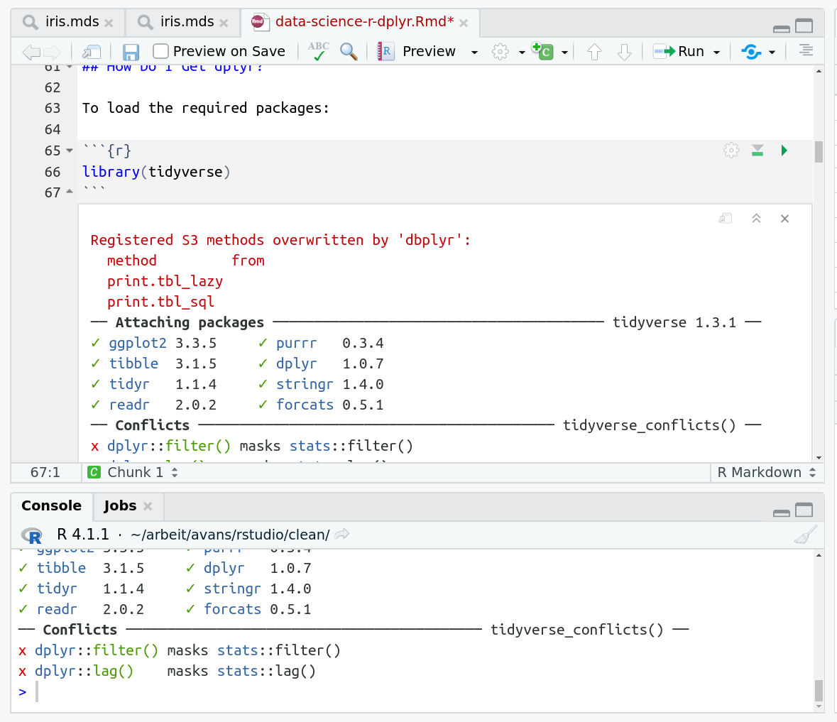
When you run cells, the output will appear below in the Console. RStudio essentially copies the code from the RMarkdown document, to the console, and runs it, just as if you had typed it out yourself!

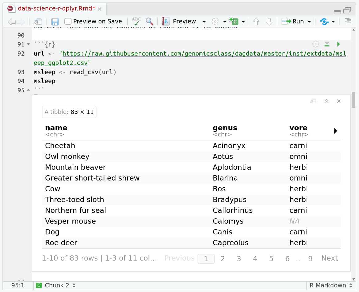
One of the best features of RMarkdown documents is that they include a very nice table browser which makes previewing results a lot easier! Instead of needing to use head every time to preview the result, you get an interactive table browser for any step which outputs a table.

In this tutorial you’ll learn to use SQL via R. Some R and SQL experience is a pre-requisite.

Comment

This tutorial is significantly based on the Carpentries Databases and SQL lesson, which is licensed CC-BY 4.0.

Abigail Cabunoc and Sheldon McKay (eds): “Software Carpentry: Using Databases and SQL.” Version 2017.08, August 2017, github.com/swcarpentry/sql-novice-survey, https://doi.org/10.5281/zenodo.838776

Adaptations have been made to make this work better in a GTN/Galaxy environment.

Agenda

In this tutorial, we will cover:

1. Programming with Databases - R
   1. Database helper functions in R

For this tutorial we need to download a database that we will use for the queries.

download.file("http://swcarpentry.github.io/sql-novice-survey/files/survey.db", destfile="survey.db")

Programming with Databases - R

Let’s have a look at how to access a database from a data analysis language like R. Other languages use almost exactly the same model: library and function names may differ, but the concepts are the same.

Here’s a short R program that selects latitudes and longitudes from an SQLite database stored in a file called survey.db:

library(RSQLite)
connection <- dbConnect(SQLite(), "survey.db")
results <- dbGetQuery(connection, "SELECT Site.lat, Site.long FROM Site;")
print(results)
dbDisconnect(connection)

The program starts by importing the RSQLite library. If we were connecting to MySQL, DB2, or some other database, we would import a different library, but all of them provide the same functions, so that the rest of our program does not have to change (at least, not much) if we switch from one database to another.

Line 2 establishes a connection to the database. Since we’re using SQLite, all we need to specify is the name of the database file. Other systems may require us to provide a username and password as well.

On line 3, we retrieve the results from an SQL query. It’s our job to make sure that SQL is properly formatted; if it isn’t, or if something goes wrong when it is being executed, the database will report an error. This result is a dataframe with one row for each entry and one column for each column in the database.

Finally, the last line closes our connection, since the database can only keep a limited number of these open at one time. Since establishing a connection takes time, though, we shouldn’t open a connection, do one operation, then close the connection, only to reopen it a few microseconds later to do another operation. Instead, it’s normal to create one connection that stays open for the lifetime of the program.

Queries in real applications will often depend on values provided by users. For example, this function takes a user’s ID as a parameter and returns their name:

library(RSQLite)

connection <- dbConnect(SQLite(), "survey.db")

getName <- function(personID) {
  query <- paste0("SELECT personal || ' ' || family FROM Person WHERE id =='",
                  personID, "';")
  return(dbGetQuery(connection, query))
}

print(paste("full name for dyer:", getName('dyer')))

dbDisconnect(connection)

We use string concatenation on the first line of this function to construct a query containing the user ID we have been given. This seems simple enough, but what happens if someone gives us this string as input?

dyer'; DROP TABLE Survey; SELECT '

It looks like there’s garbage after the user’s ID, but it is very carefully chosen garbage. If we insert this string into our query, the result is:

SELECT personal || ' ' || family FROM Person WHERE id='dyer'; DROP TABLE Survey; SELECT '';

If we execute this, it will erase one of the tables in our database.

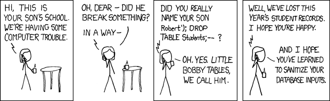
This is called an SQL injection attack, and it has been used to attack thousands of programs over the years. In particular, many web sites that take data from users insert values directly into queries without checking them carefully first. A very relevant XKCD that explains the dangers of using raw input in queries a little more succinctly:

Since an unscrupulous parent might try to smuggle commands into our queries in many different ways, the safest way to deal with this threat is to replace characters like quotes with their escaped equivalents, so that we can safely put whatever the user gives us inside a string. We can do this by using a prepared statement instead of formatting our statements as strings. Here’s what our example program looks like if we do this:

library(RSQLite)
connection <- dbConnect(SQLite(), "survey.db")

getName <- function(personID) {
  query <- "SELECT personal || ' ' || family FROM Person WHERE id == ?"
  return(dbGetPreparedQuery(connection, query, data.frame(personID)))
}

print(paste("full name for dyer:", getName('dyer')))

dbDisconnect(connection)

The key changes are in the query string and the dbGetQuery call (we use dbGetPreparedQuery instead). Instead of formatting the query ourselves, we put question marks in the query template where we want to insert values. When we call dbGetPreparedQuery, we provide a dataframe that contains as many values as there are question marks in the query. The library matches values to question marks in order, and translates any special characters in the values into their escaped equivalents so that they are safe to use.

Question: Filling a Table vs. Printing Values

Write an R program that creates a new database in a file called original.db containing a single table called Pressure, with a single field called reading, and inserts 100,000 random numbers between 10.0 and 25.0. How long does it take this program to run? How long does it take to run a program that simply writes those random numbers to a file?

Question: Filtering in SQL vs. Filtering in R

Write an R program that creates a new database called backup.db with the same structure as original.db and copies all the values greater than 20.0 from original.db to backup.db. Which is faster: filtering values in the query, or reading everything into memory and filtering in R?

Database helper functions in R

R’s database interface packages (like RSQLite) all share a common set of helper functions useful for exploring databases and reading/writing entire tables at once.

To view all tables in a database, we can use dbListTables():

connection <- dbConnect(SQLite(), "survey.db")
dbListTables(connection)

To view all column names of a table, use dbListFields():

dbListFields(connection, "Survey")

To read an entire table as a dataframe, use dbReadTable():

dbReadTable(connection, "Person")

Finally to write an entire table to a database, you can use dbWriteTable(). Note that we will always want to use the row.names = FALSE argument or R will write the row names as a separate column. In this example we will write R’s built-in iris dataset as a table in survey.db.

dbWriteTable(connection, "iris", iris, row.names = FALSE)
head(dbReadTable(connection, "iris"))

And as always, remember to close the database connection when done!

dbDisconnect(connection)

Key points

• Data analysis languages have libraries for accessing databases.

• To connect to a database, a program must use a library specific to that database manager.

• R’s libraries can be used to directly query or read from a database.

• Programs can read query results in batches or all at once.

• Queries should be written using parameter substitution, not string formatting.

• R has multiple helper functions to make working with databases easier.

Frequently Asked Questions

Feedback

Did you use this material as an instructor? Feel free to give us feedback on how it went.
Did you use this material as a learner or student? Click the form below to leave feedback.

Citing this Tutorial

1. carpentries, Helena Rasche, avans-atgm, SQL with R (Galaxy Training Materials). https://training.galaxyproject.org/training-material/topics/data-science/tutorials/sql-r/tutorial.html Online; accessed TODAY
2. Hiltemann, Saskia, Rasche, Helena et al., 2023 Galaxy Training: A Powerful Framework for Teaching! PLOS Computational Biology 10.1371/journal.pcbi.1010752
3. Batut et al., 2018 Community-Driven Data Analysis Training for Biology Cell Systems 10.1016/j.cels.2018.05.012

BibTeX

@misc{data-science-sql-r,
author = "carpentries and Helena Rasche and avans-atgm",
	title = "SQL with R (Galaxy Training Materials)",
	year = "",
	month = "",
	day = ""
	url = "\url{https://training.galaxyproject.org/training-material/topics/data-science/tutorials/sql-r/tutorial.html}",
	note = "[Online; accessed TODAY]"
}
@article{Hiltemann_2023,
	doi = {10.1371/journal.pcbi.1010752},
	url = {https://doi.org/10.1371%2Fjournal.pcbi.1010752},
	year = 2023,
	month = {jan},
	publisher = {Public Library of Science ({PLoS})},
	volume = {19},
	number = {1},
	pages = {e1010752},
	author = {Saskia Hiltemann and Helena Rasche and Simon Gladman and Hans-Rudolf Hotz and Delphine Larivi{\`{e}}re and Daniel Blankenberg and Pratik D. Jagtap and Thomas Wollmann and Anthony Bretaudeau and Nadia Gou{\'{e}} and Timothy J. Griffin and Coline Royaux and Yvan Le Bras and Subina Mehta and Anna Syme and Frederik Coppens and Bert Droesbeke and Nicola Soranzo and Wendi Bacon and Fotis Psomopoulos and Crist{\'{o}}bal Gallardo-Alba and John Davis and Melanie Christine Föll and Matthias Fahrner and Maria A. Doyle and Beatriz Serrano-Solano and Anne Claire Fouilloux and Peter van Heusden and Wolfgang Maier and Dave Clements and Florian Heyl and Björn Grüning and B{\'{e}}r{\'{e}}nice Batut and},
	editor = {Francis Ouellette},
	title = {Galaxy Training: A powerful framework for teaching!},
	journal = {PLoS Comput Biol} Computational Biology}
}

                   

Go Further

Do you want to extend your knowledge? Follow one of our recommended follow-up trainings:

Galaxy Administrators: Install the missing tools

You can use Ephemeris's shed-tools install command to install the tools used in this tutorial.

shed-tools install [-g GALAXY] [-a API_KEY] -t <(curl https://training.galaxyproject.org/training-material/api/topics/data-science/tutorials/sql-r/tutorial.json | jq .admin_install_yaml -r)

Alternatively you can copy and paste the following YAML

---
install_tool_dependencies: true
install_repository_dependencies: true
install_resolver_dependencies: true
tools: []

Feedback