Traditional dimensionality reduction techniques, while useful, often fail to capture the complex non-linear relationships present in high-dimensional data. Deep learning approaches, particularly Variational Autoencoders (VAEs), have emerged as powerful tools for unsupervised analysis of single-cell transcriptomic data (Zhao et al. 2017). VAEs combine the representational power of neural networks with probabilistic modeling, enabling them to learn meaningful latent representations while accounting for the inherent uncertainty in biological data. The key advantage of VAEs lies in their ability to encode high-dimensional gene expression profiles into a lower-dimensional latent space that preserves the most informative biological variation. This latent representation can then be used for various downstream analyses, including clustering, trajectory inference, and data integration.

Flexynesis represents a state-of-the-art deep learning framework specifically designed for multi-modal data integration in biological research (Uyar et al. 2024). What sets Flexynesis apart is its comprehensive suite of deep learning architectures, including supervised and unsupervised VAEs, that can handle various data integration scenarios while providing robust feature selection and hyperparameter optimization.

When an outcome variable is not available, or it is desired to do an unsupervised training, the supervised_vae model in flexynesis can be utilized. The supervised variational autoencoder class can be trained on the input dataset without a supervisor head. If the user passes no target variables, batch variables, or survival variables, then the class behaves as a plain variational autoencoder.

This training is inspired from the original flexynesis analysis notebook: unsupervised_analysis_single_cell.ipynb.

Here, we demonstrate the capabilities of flexynesis on a Single-cell CITE-Seq dataset of Bone Marrow samples (Stuart et al. 2019). The dataset was downloaded and processed using Seurat (v5.1.0) (Hao et al. 2021). 5000 cells were randomly sampled for training and 5000 cells were sampled for testing.

Warning: LICENSE

Flexynesis is only available for NON-COMMERCIAL use. Permission is only granted for academic, research, and educational purposes. Before using, be sure to review, agree, and comply with the license. For commercial use, please review the flexynesis license on GitHub and contact the copyright holders

Agenda

In this tutorial, we will cover:

1. Data upload
   1. Get data
2. Unsupervised Training of Flexynesis
3. Clustering and visualisation
   1. Louvain clustering
   2. Get optimal clusters
   3. Compute AMI, ARI
   4. UMAP visualisation of true and Louvain lables
4. Conclusion

Data upload

In the first part of this tutorial we will upload processed CITE-seq data from bone marrow tissue.

All data are in tabular format and they include:

• ADT (Antibody-Derived Tags which indicates the quantification of cell surface proteins) data
• RNA expression data
• Clinical data includes some information about each cell like number of RNAs, genes, … (In next steps we will use the clustering information “celltype_l2”)

Get data

Hands On: Data Upload

1. Create a new history for this tutorial

   Tip: Creating a new history

   To create a new history simply click the new-history icon at the top of the history panel:

   

2. Import the files from Zenodo:

   https://zenodo.org/records/16287482/files/test-ADT_BMscRNAseq.tabular
   https://zenodo.org/records/16287482/files/test-clin_BMscRNAseq.tabular
   https://zenodo.org/records/16287482/files/test-RNA_BMscRNAseq.tabular
   https://zenodo.org/records/16287482/files/train-ADT_BMscRNAseq.tabular
   https://zenodo.org/records/16287482/files/train-clin_BMscRNAseq.tabular
   https://zenodo.org/records/16287482/files/train-RNA_BMscRNAseq.tabular
   

   Tip: Importing via links

   • Copy the link location

   • Click galaxy-upload Upload Data at the top of the tool panel

   • Select galaxy-wf-edit Paste/Fetch Data

   • Paste the link(s) into the text field

   • Press Start

   • Close the window

3. Rename the datasets

4. Check that the datatype is tabular

   Tip: Changing the datatype

   • Click on the galaxy-pencil pencil icon for the dataset to edit its attributes
   • In the central panel, click galaxy-chart-select-data Datatypes tab on the top
   • In the galaxy-chart-select-data Assign Datatype, select tabular from “New Type” dropdown
     • Tip: you can start typing the datatype into the field to filter the dropdown menu
   • Click the Save button

5. Add to each dataset a representative tag (RNA, ADT, clin)

   Tip: Adding a tag

   Datasets can be tagged. This simplifies the tracking of datasets across the Galaxy interface. Tags can contain any combination of letters or numbers but cannot contain spaces.

   To tag a dataset:

   1. Click on the dataset to expand it
   2. Click on Add Tags galaxy-tags
   3. Add tag text. Tags starting with # will be automatically propagated to the outputs of tools using this dataset (see below).
   4. Press Enter
   5. Check that the tag appears below the dataset name

   Tags beginning with # are special!

   They are called Name tags. The unique feature of these tags is that they propagate: if a dataset is labelled with a name tag, all derivatives (children) of this dataset will automatically inherit this tag (see below). The figure below explains why this is so useful. Consider the following analysis (numbers in parenthesis correspond to dataset numbers in the figure below):

   1. a set of forward and reverse reads (datasets 1 and 2) is mapped against a reference using Bowtie2 generating dataset 3;
   2. dataset 3 is used to calculate read coverage using BedTools Genome Coverage separately for + and - strands. This generates two datasets (4 and 5 for plus and minus, respectively);
   3. datasets 4 and 5 are used as inputs to Macs2 broadCall datasets generating datasets 6 and 8;
   4. datasets 6 and 8 are intersected with coordinates of genes (dataset 9) using BedTools Intersect generating datasets 10 and 11.

   

   Now consider that this analysis is done without name tags. This is shown on the left side of the figure. It is hard to trace which datasets contain “plus” data versus “minus” data. For example, does dataset 10 contain “plus” data or “minus” data? Probably “minus” but are you sure? In the case of a small history like the one shown here, it is possible to trace this manually but as the size of a history grows it will become very challenging.

   The right side of the figure shows exactly the same analysis, but using name tags. When the analysis was conducted datasets 4 and 5 were tagged with #plus and #minus, respectively. When they were used as inputs to Macs2 resulting datasets 6 and 8 automatically inherited them and so on… As a result it is straightforward to trace both branches (plus and minus) of this analysis.

   More information is in a dedicated #nametag tutorial.

Unsupervised Training of Flexynesis

Hands On: Train unsupervised model

1. Flexynesis ( Galaxy version 0.2.20+galaxy3) with the following parameters:
   • “I certify that I am not using this tool for commercial purposes.”: Yes
   • “Type of Analysis”: Unsupervised Training
     • param-file “Training clinical data”: train-clin_BMscRNAseq.tabular
     • param-file “Test clinical data”: test-clin_BMscRNAseq.tabular
     • param-file “Training omics data”: train-RNA_BMscRNAseq.tabular
     • param-file “Test omics data”: test-RNA_BMscRNAseq.tabular
     • “What type of assay is your input?”: RNA
     • In “Multiple omics layers?”:
       • param-repeat “Insert Multiple omics layers?”
         • param-file “Training omics data”: train-ADT_BMscRNAseq.tabular
         • param-file “Test omics data”: test-ADT_BMscRNAseq.tabular
         • “What type of assay is your input?”: ADT
     • In “Advanced Options”:
       • “How many epochs to wait when no improvements in validation loss are observed.”: 5
       • “Number of iterations for hyperparameter optimization.”: 1

   Comment: Advanced options

   In this tutorial, for the sake of time, we are using 1 iteration for hyperparameter optimization. In a real-life analysis you might want to increase this number according to your dataset.

Question

1. What are the outputs from Flexynesis?

Solution

1. There are two tabular files for the latent space embeddings and two feature log files for each of the modalities.

Clustering and visualisation

Now, we extract the sample embeddings from the test dataset, cluster the cells using Louvain clustering, and visualize the clusters along with known cell type labels.

Hands On: Extract test embeddings

1. Extract dataset with the following parameters:
   • param-file “Input List”: results (output of Flexynesis tool)
   • “How should a dataset be selected?”: The first dataset

Question

1. What are other options to extract datasets from a collection?

Solution

1. It is also possible to use index (here index 0) or data name (here job.embeddings_test) to extract the data. Please always check your collection before extraction.

Louvain clustering

Hands On: Cluster cells by Louvain method

1. Flexynesis utils ( Galaxy version 0.2.20+galaxy3) with the following parameters:
   • “I certify that I am not using this tool for commercial purposes.”: Yes
   • “Flexynesis utils”: Louvain Clustering
     • param-file “Matrix”: job.embeddings_test (output of Extract dataset tool)
     • param-file “Predicted labels”: test-clin_BMscRNAseq.tabular (Input dataset)
     • “Number of nearest neighbors to connect for each node”: 15

Question

1. What is the output of this tool?

Solution

1. The output is the test-clin_BMscRNAseq.tabular file with a column added containing Louvain clustering values.

Get optimal clusters

Now we will use k-means clustering with a varying number of expected clusters and pick the best one based on silhouette scores.

Hands On: Get optimal clusters

1. Flexynesis utils ( Galaxy version 0.2.20+galaxy3) with the following parameters:
   • “I certify that I am not using this tool for commercial purposes.”: Yes
   • “Flexynesis utils”: Get Optimal Clusters
     • param-file “Matrix”: job.embeddings_test (output of Extract dataset tool)
     • param-file “Predicted labels”: louvain_clustering (output of Flexynesis utils tool)
     • “Minimum number of clusters to try”: 5
     • “Maximum number of clusters to try”: 15

   Comment: Predicted labels

   Please make sure to use the output of Louvain clustering. We need those values in one table for next steps.

2. Rename the output to labels with optimal clusters

Question

1. What is the output of this tool?

Solution

1. Another column is added to the previous table for k-means clustering values.

In the next step, we will calculate the concrdance between the known cell types and unsupervised cluster labels using AMI (Adjusted Mutual Information) and ARI (Adjusted Rand Index) indices.

Compute AMI, ARI

AMI (Adjusted Mutual Information) and ARI (Adjusted Rand Index) are used to compare clustering results with ground truth labels. They measure concordance (agreement) between two clusterings. AMI ranges from 0 (no agreement) to 1 (perfect match) and ARI ranges from -1 (complete disagreement) to 1 (perfect agreement).

Hands On: Louvain vs true labels

1. Flexynesis utils ( Galaxy version 0.2.20+galaxy3) with the following parameters:
   • “I certify that I am not using this tool for commercial purposes.”: Yes
   • “Flexynesis utils”: Compute AMI and ARI
     • param-file “Predicted labels”: labels with optimal clusters (output of Flexynesis utils tool)
     • “Column name in the labels file to use for the true labels”: c10 (celltype_l2)
     • “Column name in the labels file to use for the predicted labels”: c12 (louvain_cluster)

Hands On: k-means vs true labels

1. Flexynesis utils ( Galaxy version 0.2.20+galaxy3) with the following parameters:
   • “I certify that I am not using this tool for commercial purposes.”: Yes
   • “Flexynesis utils”: Compute AMI and ARI
     • param-file “Predicted labels”: labels with optimal clusters (output of Flexynesis utils tool)
     • “Column name in the labels file to use for the true labels”: c10 (celltype_l2)
     • “Column name in the labels file to use for the predicted labels”: c13 (optimal_kmeans_cluster)

Question

1. Which of the clusterings has better concordance with the known cell type? Louvain and k-means?

Solution

1. The Louvain has AMI = 0.66 and ARI = 0.49 and k-means has AMI = 0.55 and ARI = 0.43. Louvain Clustering seems to yield better AMI/ARI scores. So, we use them to do more visualizations.

UMAP visualisation of true and Louvain lables

Hands On: Dimension reduction plot

1. Flexynesis plot ( Galaxy version 0.2.20+galaxy3) with the following parameters:
   • “I certify that I am not using this tool for commercial purposes.”: Yes
   • “Flexynesis plot”: Dimensionality reduction
     • param-file “Embeddings”: job.embeddings_test (output of Extract dataset tool)
     • param-file “Predicted labels”: labels with optimal clusters (output of Flexynesis utils tool)
     • “Column in the labels file to use for coloring the points in the plot”: c10 (celltype_l2)
     • “Transformation method”: UMAP

Hands On: Dimension reduction plot

1. Flexynesis plot ( Galaxy version 0.2.20+galaxy3) with the following parameters:
   • “I certify that I am not using this tool for commercial purposes.”: Yes
   • “Flexynesis plot”: Dimensionality reduction
     • param-file “Predicted labels”: labels with optimal clusters (output of Flexynesis utils tool)
     • “Column in the labels file to use for coloring the points in the plot”: c12 (louvain_cluster)
     • “Transformation method”: UMAP

Question

1. Compare these two UMAP plots, Is the unsupervised clustering close to the ground truth labels?

Solution

1. We can see that like true labels, each UMAP clusters have unique Louvain clusters assigned. This shows that this clustering based on the latent space is close to the ground truth. However, we still don’t know which Louvain cluster, corresponds to which true label.

Open image in new tab

Open image in new tab

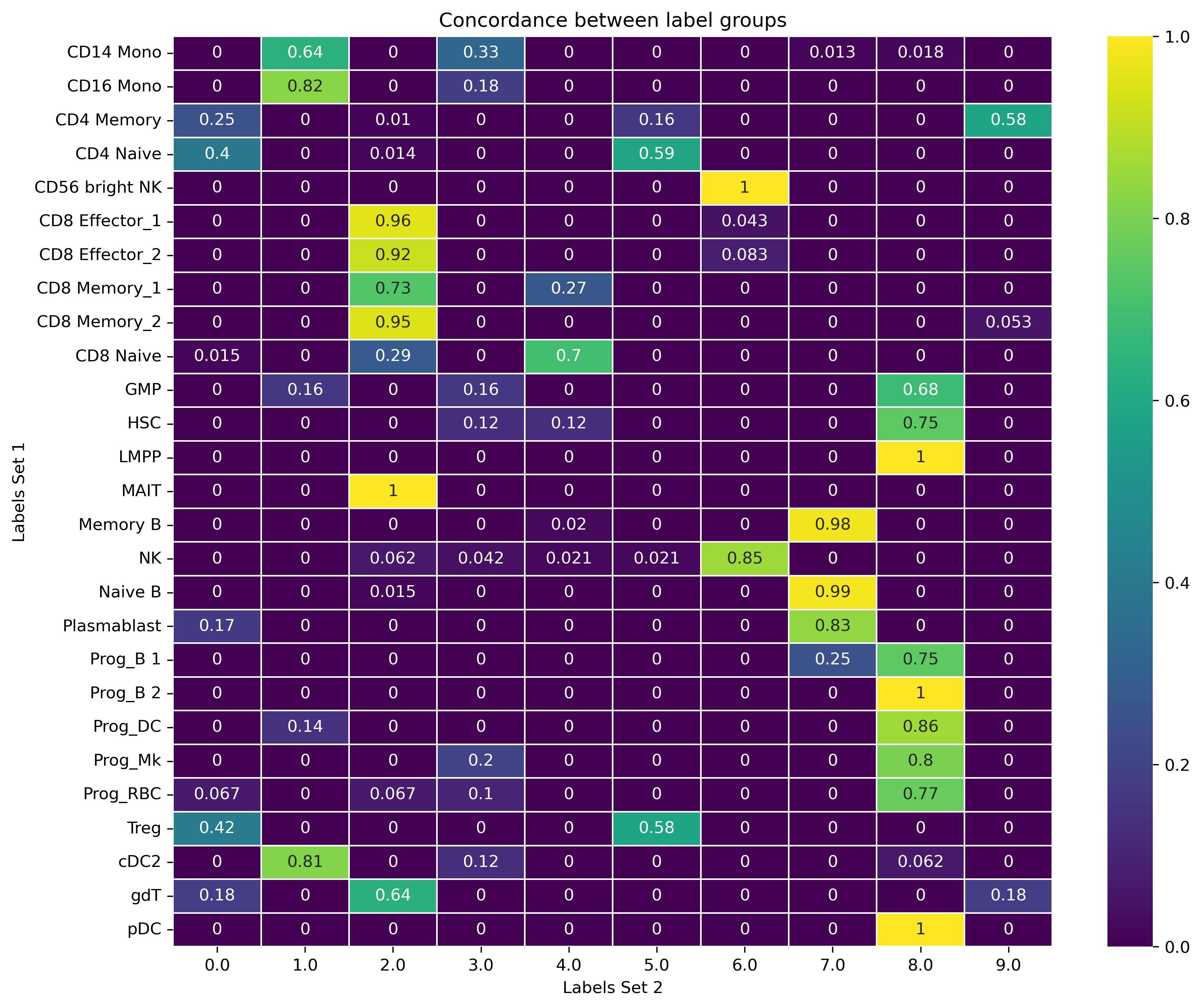
To see the real concordance between Louvain clusters and true values, we can observe a tabulation of the concordance between them. (Each row sums up to 1).

Hands On: Concordance plot

1. Flexynesis plot ( Galaxy version 0.2.20+galaxy3) with the following parameters:
   • “I certify that I am not using this tool for commercial purposes.”: Yes
   • “Flexynesis plot”: Label concordance heatmap
     • param-file “Predicted labels”: labels with optimal clusters (output of Flexynesis utils tool)
     • “Column in the labels file to use for true labels”: c10 (celltype_l2)
     • “Column in the labels file to use for predicted labels”: c12 (louvain_cluster)

Now it is easier to see which Lovain cluster corresponds to which true value.

Open image in new tab

Conclusion

Here we demonstrated the power of Flexynesis for unsupervised analysis of multi-modal single-cell data. We explored how variational autoencoders can capture cellular heterogeneity without requiring labeled training data.

You've Finished the Tutorial

Please also consider filling out the Feedback Form as well!

Key points

• Variational autoencoders can effectively capture cellular heterogeneity in single-cell data without requiring labeled training data

• Flexynesis provides a structured framework for multi-modal data integration with rigorous evaluation procedures

• Unsupervised feature learning can reveal biologically meaningful cellular populations and relationships

• Low-dimensional embeddings from VAEs can be used for clustering, visualization, and biological interpretation

Frequently Asked Questions

• Tutorial FAQs
• Topic FAQs
• Galaxy FAQs
• GTN Matrix Chat
• Galaxy Help Forum

References

1. Zhao, S., J. Song, and S. Ermon, 2017 InfoVAE: Information Maximizing Variational Autoencoders. CoRR abs/1706.02262: http://arxiv.org/abs/1706.02262
2. Stuart, T., A. Butler, P. Hoffman, C. Hafemeister, E. Papalexi et al., 2019 Comprehensive Integration of Single-Cell Data. Cell 177: 1888–1902.e21. 10.1016/j.cell.2019.05.031
3. Hao, Y., S. Hao, E. Andersen-Nissen, W. M. Mauck, S. Zheng et al., 2021 Integrated analysis of multimodal single-cell data. Cell 184: 3573–3587.e29. 10.1016/j.cell.2021.04.048
4. Uyar, B., T. Savchyn, R. Wurmus, A. Sarigun, M. M. Shaik et al., 2024 Flexynesis: A deep learning framework for bulk multi-omics data integration for precision oncology and beyond. 10.1101/2024.07.16.603606

Feedback

Did you use this material as an instructor? Feel free to give us feedback on how it went.
Did you use this material as a learner or student? Click the form below to leave feedback.

Citing this Tutorial

1. Amirhossein Naghsh Nilchi, Björn Grüning, Unsupervised Analysis of Bone Marrow Cells with Flexynesis (Galaxy Training Materials). https://training.galaxyproject.org/training-material/topics/statistics/tutorials/flexynesis_unsupervised/tutorial.html Online; accessed TODAY
2. Hiltemann, Saskia, Rasche, Helena et al., 2023 Galaxy Training: A Powerful Framework for Teaching! PLOS Computational Biology 10.1371/journal.pcbi.1010752
3. Batut et al., 2018 Community-Driven Data Analysis Training for Biology Cell Systems 10.1016/j.cels.2018.05.012

BibTeX

@misc{statistics-flexynesis_unsupervised,
author = "Amirhossein Naghsh Nilchi and Björn Grüning",
	title = "Unsupervised Analysis of Bone Marrow Cells with Flexynesis (Galaxy Training Materials)",
	year = "",
	month = "",
	day = "",
	url = "\url{https://training.galaxyproject.org/training-material/topics/statistics/tutorials/flexynesis_unsupervised/tutorial.html}",
	note = "[Online; accessed TODAY]"
}
@article{Hiltemann_2023,
	doi = {10.1371/journal.pcbi.1010752},
	url = {https://doi.org/10.1371%2Fjournal.pcbi.1010752},
	year = 2023,
	month = {jan},
	publisher = {Public Library of Science ({PLoS})},
	volume = {19},
	number = {1},
	pages = {e1010752},
	author = {Saskia Hiltemann and Helena Rasche and Simon Gladman and Hans-Rudolf Hotz and Delphine Larivi{\`{e}}re and Daniel Blankenberg and Pratik D. Jagtap and Thomas Wollmann and Anthony Bretaudeau and Nadia Gou{\'{e}} and Timothy J. Griffin and Coline Royaux and Yvan Le Bras and Subina Mehta and Anna Syme and Frederik Coppens and Bert Droesbeke and Nicola Soranzo and Wendi Bacon and Fotis Psomopoulos and Crist{\'{o}}bal Gallardo-Alba and John Davis and Melanie Christine Föll and Matthias Fahrner and Maria A. Doyle and Beatriz Serrano-Solano and Anne Claire Fouilloux and Peter van Heusden and Wolfgang Maier and Dave Clements and Florian Heyl and Björn Grüning and B{\'{e}}r{\'{e}}nice Batut and},
	editor = {Francis Ouellette},
	title = {Galaxy Training: A powerful framework for teaching!},
	journal = {PLoS Comput Biol}
}

                   

Galaxy Administrators: Install the missing tools

You can use Ephemeris's shed-tools install command to install the tools used in this tutorial.

shed-tools install [-g GALAXY] [-a API_KEY] -t <(curl https://training.galaxyproject.org/training-material/api/topics/statistics/tutorials/flexynesis_unsupervised/tutorial.json | jq .admin_install_yaml -r)

Alternatively you can copy and paste the following YAML

---
install_tool_dependencies: true
install_repository_dependencies: true
install_resolver_dependencies: true
tools: []

Feedback

No feedback has been recieved yet for this training. Be the first one by filling in the feedback form.