Binning of metagenomic sequencing data
| Author(s) |
|
| Editor(s) |
|
| Reviewers |
|
OverviewQuestions:
Objectives:
What is metagenomic binning refers to?
Which tools may be used for metagenomic binning?
How to assess the quality of metagenomic binning?
Requirements:
Describe what is metagenomics binning.
Describe common challenges in metagenomics binning.
Perform metagenomic binning using MetaBAT 2 software.
Evaluation of MAG quality and completeness using CheckM software.
Time estimation: 2 hoursLevel: Intermediate IntermediateSupporting Materials:Published: Dec 5, 2023Last modification: Apr 9, 2026License: Tutorial Content is licensed under Creative Commons Attribution 4.0 International License. The GTN Framework is licensed under MITpurl PURL: https://gxy.io/GTN:T00387rating Rating: 4.0 (1 recent ratings, 11 all time)version Revision: 9
Metagenomics is the study of genetic material recovered directly from environmental samples, such as soil, water, or gut contents, without the need for isolating or cultivating individual organisms. Metagenomics binning is a process used to classify DNA sequences obtained from metagenomic sequencing into discrete groups, or bins, based on their similarity to each other.
The goal of metagenomics binning is to assign DNA sequences to the organisms or taxonomic groups from which they originate, allowing for a better understanding of the diversity and functions of the microbial communities present in the sample. This is typically achieved through computational methods that include sequence similarity, composition, and other features to group the sequences into bins.
CommentBefore starting this tutorial, it is recommended to do the Metagenomics Assembly Tutorial
Binning approaches
There are several approaches to metagenomics binning, including:
-
Sequence composition-based binning: This method is based on the observation that different genomes have distinct sequence composition patterns, such as GC content or codon usage bias. By analyzing these patterns in metagenomic data, sequence fragments can be assigned to individual genomes or groups of genomes.
-
Coverage-based binning: This method uses the depth of coverage of sequencing reads to group them into bins. Sequencing reads that originate from the same genome are expected to have similar coverage, and this information can be used to identify groups of reads that represent individual genomes or genome clusters.
-
Hybrid binning: This method combines sequence composition-based and coverage-based binning to increase the accuracy of binning results. By using multiple sources of information, hybrid binning can better distinguish closely related genomes that may have similar sequence composition patterns.
-
Clustering-based binning: This method groups sequence fragments into clusters based on sequence similarity, and then assigns each cluster to a genome or genome cluster based on its sequence composition and coverage. This method is particularly useful for metagenomic data sets with high levels of genomic diversity.
-
Supervised machine learning-based binning: This method uses machine learning algorithms trained on annotated reference genomes to classify metagenomic data into bins. This approach can achieve high accuracy but requires a large number of annotated genomes for training.
Binning challenges
Metagenomic binning is a complex process that involves many steps and can be challenging due to several problems that can occur during the process. Some of the most common problems encountered in metagenomic binning include:
- High complexity: Metagenomic samples contain DNA from multiple organisms, which can lead to high complexity in the data.
- Fragmented sequences: Metagenomic sequencing often generates fragmented sequences, which can make it difficult to assign reads to the correct bin.
- Uneven coverage: Some organisms in a metagenomic sample may be more abundant than others, leading to uneven coverage of different genomes.
- Incomplete or partial genomes: Metagenomic sequencing may not capture the entire genome of a given organism, which can make it difficult to accurately bin sequences from that organism.
- Horizontal gene transfer: Horizontal gene transfer (HGT) can complicate metagenomic binning, as it can introduce genetic material from one organism into another.
- Chimeric sequences: Sequences that are the result of sequencing errors or contamination can lead to chimeric sequences, which can make it difficult to accurately bin reads.
- Strain variation: Organisms within a species can exhibit significant genetic variation, which can make it difficult to distinguish between different strains in a metagenomic sample.
Common binners
There are different algorithms and tools performing metagenomic binning. The most widely used include:
- MaxBin (Wu et al. 2015): A popular de novo binning algorithm that uses a combination of sequence features and marker genes to cluster contigs into genome bins.
- MetaBAT (Kang et al. 2019): Another widely used de novo binning algorithm that employs a hierarchical clustering approach based on tetranucleotide frequency and coverage information.
- CONCOCT (Alneberg et al. 2014): A de novo binning tool that uses a clustering algorithm based on sequence composition and coverage information to group contigs into genome bins.
- MyCC (Lin and Liao 2016): A reference-based binning tool that uses sequence alignment to identify contigs belonging to the same genome or taxonomic group.
- GroopM (Imelfort et al. 2014): A hybrid binning tool that combines reference-based and de novo approaches to achieve high binning accuracy.
- SemiBin (Pan et al. 2022): A command-line tool for metagenomic binning with deep learning, handling both short and long reads.
- Vamb (Nissen et al. 2021): An algorithm that uses variational autoencoders (VAEs) to encode sequence composition and coverage information.
- ComeBin (Wang et al. 2024): A metagenomic binning tool that integrates both composition and abundance features with machine learning-based clustering to improve binning accuracy across complex microbial communities.
So many options, what binner to use ?
Each of these binning methods has its own strengths and limitations, and the choice of a binning tool often depends on the characteristics of the metagenomic dataset and the research question. Practical guidance on which binner to use for specific datasets and environments can be drawn from benchmark studies such as Author et al. 2025.
 Open image in new tab
Another useful approach to investigate the performance of binners is to use simulated datasets. Therefore, the CAMI challenges (Meyer et al. 2022) were introduced. CAMI, which stands for Critical Assessment of Metagenome Interpretation, is an international community-driven initiative that organizes benchmarking challenges to objectively evaluate the performance of metagenomic tools. This includes the benchmarking of binners based on standardized, realistically simulated microbial communities that vary in complexity, strain diversity, and abundance.
 Open image in new tab
A general approach is to perform binning using multiple binners that have shown good performance for the specific dataset, followed by bin refinement to generate an improved bin set that retains the best bins from the analysis.
Does using more binners always improve results? In practice, one must also consider computational resources and time constraints. Running many binners can be very time-consuming and resource-intensive, especially for large studies. In some cases, adding extra binners does not lead to a meaningful increase in bin quality, so the choice of binners should be made carefully. Overall, identifying the optimal combination of binners remains an active area of research, and clear, widely accepted guidelines are still being established.
Bin refinement
There are also bin refinement tools, which can evaluate, combine, and improve the raw bins produced by primary binners such as MetaBAT2, CONCOCT, MaxBin2, or SemiBin. These tools help remove contamination, merge complementary bins, and recover higher-quality MAGs.
-
MetaWRAP (Uritskiy et al. 2018): A comprehensive metagenomic analysis pipeline that includes modules for quality control, assembly, binning (wrapping multiple binners), refinement, reassembly, and annotation. It provides an easy-to-use framework for producing high-quality MAGs from raw reads.
-
DAS Tool (Sieber et al. 2018): A bin-refinement tool that combines results from multiple binners (e.g., MetaBAT2, MaxBin2, CONCOCT, SemiBin) into a consensus set of optimized, non-redundant bins. DAS Tool improves overall bin quality by integrating the strengths from several algorithms.
-
Binnette (Mainguy and Hoede 2024): A fast and accurate bin refinement tool that constructs high-quality MAGs from the outputs of multiple binning tools. It generates hybrid bins using set operations on overlapping contigs — intersection, difference, and union — and evaluates their quality with CheckM2 to select the best bins. Compared to metaWRAP, Binette is faster and can process an unlimited number of input bin sets, making it highly scalable for large and complex metagenomic datasets.
Anvi’o (Eren et al. 2015) is a platform for interactive visualization and manual refinement of metagenomic bins. While it can run automated binning (defaulting to CONCOCT), its main strength lies in allowing users to:
- Inspect contig-level coverage, GC content, and single-copy gene presence
- Visualize connections between contigs in a network view
- Manually merge, split, or reassign contigs to improve bin completeness and reduce contamination
- Annotate bins and link them to taxonomic or functional information
This interactive approach is particularly useful when automated binning produces ambiguous or low-quality bins, enabling high-confidence MAG reconstruction.
Mock binning dataset for this training
Read mapping and binning real metagenomic datasets is a computationally demanding and time-consuming task. To demonstrate the basics of binning in this tutorial, we generated a small mock dataset that is just large enough to produce bins for all binners in this tutorial. The same binners can be applied for any real-life datasets, but as said, plan in some time, up to weeks in some cases.
AgendaIn this tutorial, we will cover:
Prepare analysis history and data
Metagenomic binners typically take two types of data as input:
-
A fasta file containing the assembled contigs, which can be generated from raw metagenomic sequencing reads using an assembler such as MEGAHIT, SPAdes, or IDBA-UD.
-
A BAM file containing the read coverage information for each contig, which can be generated from the same sequencing reads using mapping software such as Bowtie2 or BWA.
Comment: Can Bins be generated without coverage information?Not all binners require coverage information. Some, like MetaBAT2, can operate using only genomic composition (e.g., tetranucleotide frequencies) when coverage files are not available. This is especially useful for single-sample datasets or legacy data where coverage cannot easily be calculated.
Other tools that support composition-only binning include:
- MaxBin 2, which can run with composition alone, but performs better with depth.
- SolidBin, which supports single-sample binning based on sequence features.
- VAMB, which primarily uses deep learning on composition, coverage optional.
That said, including coverage information generally increases binning accuracy, especially for:
- Differentiating closely related strains
- Datasets with uneven abundance
- Multi-sample metagenomics workflows (e.g., differential coverage binning)
In summary: yes, it’s possible to bin without coverage, but coverage-aware workflows are recommended when available, as they reduce contamination and improve completeness.
To run binning, we first need to get the data into Galaxy. Any analysis should get its own Galaxy history. So let’s start by creating a new one:
Hands On: Prepare the Galaxy history
Create a new history for this analysis
To create a new history simply click the new-history icon at the top of the history panel:
Rename the history
- Click on galaxy-pencil (Edit) next to the history name (which by default is “Unnamed history”)
- Type the new name
- Click on Save
- To cancel renaming, click the galaxy-undo “Cancel” button
If you do not have the galaxy-pencil (Edit) next to the history name (which can be the case if you are using an older version of Galaxy) do the following:
- Click on Unnamed history (or the current name of the history) (Click to rename history) at the top of your history panel
- Type the new name
- Press Enter

We need to get the data into our history.
In case of a not very large dataset it’s more convenient to upload data directly from your computer to Galaxy.
Hands On: Upload data into Galaxy
Import the contig file from Zenodo or a data library:
https://zenodo.org/records/17661262/files/MEGAHIT_contigs.fasta
- Copy the link location
Click galaxy-upload Upload at the top of the activity panel
- Select galaxy-wf-edit Paste/Fetch Data
Paste the link(s) into the text field
Press Start
- Close the window
As an alternative to uploading the data from a URL or your computer, the files may also have been made available from a shared data library:
- Go into Libraries (left panel)
- Navigate to the correct folder as indicated by your instructor.
- On most Galaxies tutorial data will be provided in a folder named GTN - Material –> Topic Name -> Tutorial Name.
- Select the desired files
- Click on Add to History galaxy-dropdown near the top and select as Datasets from the dropdown menu
In the pop-up window, choose
- “Select history”: the history you want to import the data to (or create a new one)
- Click on Import
CommentIn case of large dataset, we can use FTP server or the Galaxy Rule-based Uploader.
Create a collection named
Contigs
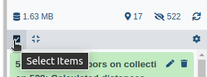
- Click on galaxy-selector Select Items at the top of the history panel
- Check all the datasets in your history you would like to include
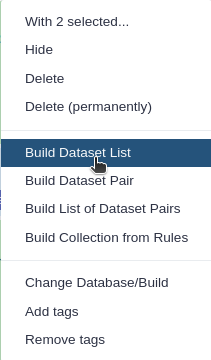
Click n of N selected and choose Advanced Build List
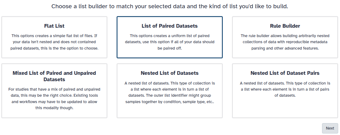
You are in collection building wizard. Choose Flat List and click ‘Next’ button at the right bottom corner.
Double clcik on the file names to edit. For example, remove file extensions or common prefix/suffixes to cleanup the names.
- Enter a name for your collection
- Click Build to build your collection
- Click on the checkmark icon at the top of your history again
Import the raw reads in fastq format from Zenodo or a data library:
https://zenodo.org/records/17661262/files/reads_forward.fastqsanger.gz
https://zenodo.org/records/17661262/files/reads_reverse.fastqsanger.gz
Create a paired collection named
Reads
- Click on galaxy-selector Select Items at the top of the history panel
- Check all the datasets in your history you would like to include
Click n of N selected and choose Advanced Build List
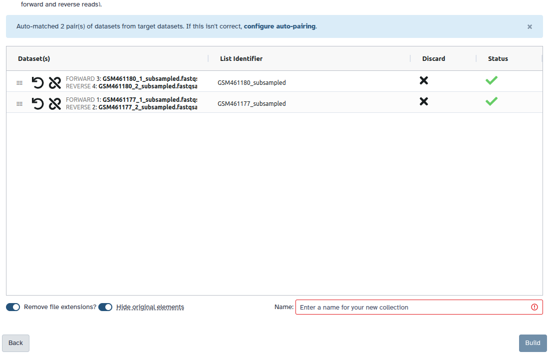
You are in the collection building wizard. Choose List of Paired Datasets and click ‘Next’ button at the right bottom corner.
Check and configure auto-pairing. Commonly matepairs have suffix
_1and_2or_R1and_R2. Click on ‘Next’ at the bottom.
- Edit the List Identifier as required.
- Enter a name for your collection
- Click Build to build your collection
- Click on the checkmark icon at the top of your history again


Comment: Why do we use collections here?In this tutorial, collections are not strictly necessary because we are working with only one contig file and its paired-end reads. However, in real metagenomic studies, it is common to process many samples—sometimes hundreds or even thousands—and in those cases, collections become essential for managing data efficiently.
It is generally good practice to first test a workflow on a small subset of the data (for example, a collection containing only a single sample) to ensure that the tools run correctly and the parameters are appropriate before launching thousands of jobs on Galaxy.
Preparation for binning
As explained before, we need coverage information in a BAM file as a requirement for all binners. Some binners need a specific format for the coverage information, but this will be covered in the version specific to the desired binner. For now, we will map the quality-controlled reads to the contigs to get a BAM file with the coverage information. This BAM file also needs to be sorted for the downstream binners.
CommentMake sure the reads are quality-controlled, e.g., by following the Quality Control tutorial
Hands On: Map reads to contigs
- Bowtie2 ( Galaxy version 2.5.4+galaxy0) with the following parameters:
- “Is this single or paired library”:
Paired-end
- param-collection “FASTQ Paired Dataset”:
Reads(Input dataset collection)- “Do you want to set paired-end options?”:
No- “Will you select a reference genome from your history or use a built-in index?”:
Use a genome from the history and build index
- param-collection “Select reference genome”:
Contigs(Input dataset collection)- “Set read groups information?”:
Do not set- “Select analysis mode”:
1: Default setting only- “Do you want to tweak SAM/BAM Options?”:
No- “Save the bowtie2 mapping statistics to the history”:
Yes
Let’s now sort the BAM files.
Hands On: Sort BAM files
- Samtools sort ( Galaxy version 2.0.7) with the following parameters:
- param-file “BAM File”: output of Bowtie2 tool
- “Primary sort key”:
coordinate
The sorted BAM file can be used as input for any of the binning tools.
Binning
As explained before, there are many challenges to metagenomics binning. The most common of them are listed below:
- High complexity.
- Fragmented sequences.
- Uneven coverage.
- Incomplete or partial genomes.
- Horizontal gene transfer.
- Chimeric sequences.
- Strain variation.
 Open image in new tab
In this tutorial, we offer several versions, each highlighting a different binners:
Hands-on: Choose Your Own TutorialThis is a 'Choose Your Own Tutorial' (CYOT) section (also known as 'Choose Your Own Analysis' (CYOA)), where you can select between multiple paths. Click one of the buttons below to select how you want to follow the tutorial
Bin contigs using MetaBAT 2
MetaBAT stands for “Metagenome Binning based on Abundance and Tetranucleotide frequency”. It is:
Grouping large fragments assembled from shotgun metagenomic sequences to deconvolute complex microbial communities, or metagenome binning, enables the study of individual organisms and their interactions. Here we developed automated metagenome binning software, called MetaBAT, which integrates empirical probabilistic distances of genome abundance and tetranucleotide frequency. On synthetic datasets MetaBAT on average achieves 98percent precision and 90% recall at the strain level with 281 near complete unique genomes. Applying MetaBAT to a human gut microbiome data set we recovered 176 genome bins with 92% precision and 80% recall. Further analyses suggest MetaBAT is able to recover genome fragments missed in reference genomes up to 19%, while 53 genome bins are novel. In summary, we believe MetaBAT is a powerful tool to facilitate comprehensive understanding of complex microbial communities.
MetaBAT is a popular software tool for metagenomics binning, and there are several reasons why it is often used:
- High accuracy: MetaBAT uses a combination of tetranucleotide frequency, coverage depth, and read linkage information to bin contigs, which has been shown to be highly accurate and efficient.
- Easy to use: MetaBAT has a user-friendly interface and can be run on a standard desktop computer, making it accessible to a wide range of researchers with varying levels of computational expertise.
- Flexibility: MetaBAT can be used with a variety of sequencing technologies, including Illumina, PacBio, and Nanopore, and can be applied to both microbial and viral metagenomes.
- Scalability: MetaBAT can handle large-scale datasets, and its performance has been shown to improve with increasing sequencing depth.
- Compatibility: MetaBAT outputs MAGs in standard formats that can be easily integrated into downstream analyses and tools, such as taxonomic annotation and functional prediction.
The first step when using tools like MetaBAT or MaxBin2 is to compute contig depths from the raw alignment data. Both tools require per-contig depth tables as input, as their binning algorithms rely on summarized coverage statistics at the contig level. However, standard BAM files store read-level alignment information, which must first be processed to generate the necessary contig-level coverage data. This preprocessing step ensures compatibility with the input requirements of these binning tools.
Hands On: Calculate contig depths
- Calculate contig depths ( Galaxy version 2.17+galaxy0) with the following parameters:
- “Mode to process BAM files”:
One by one
- param-file “Sorted bam files”: output of Samtools sort tool
- “Select a reference genome?”:
No
We can now launch the proper binning with MetaBAT 2
Hands On: Individual binning of short-reads with MetaBAT 2
- MetaBAT 2 ( Galaxy version 2.17+galaxy0) with parameters:
- “Fasta file containing contigs”:
Contigs- In Advanced options, keep all as default.
- In Output options:
- “Save cluster memberships as a matrix format?”:
"No"
MetaBAT 2 generates several output files during its execution, some of which are optional and only produced when explicitly requested by the user. These files include:
- The final set of genome bins in FASTA format (
.fa) - A summary file with information on each genome bin, including its length, completeness, contamination, and taxonomy classification (
.txt) - A file with the mapping results showing how each contig was assigned to a genome bin (
.bam) - A file containing the abundance estimation of each genome bin (
.txt) - A file with the coverage profile of each genome bin (
.txt) - A file containing the nucleotide composition of each genome bin (
.txt) - A file with the predicted gene sequences of each genome bin (
.faa)
These output files can be further analyzed and used for downstream applications such as functional annotation, comparative genomics, and phylogenetic analysis.
Question: Binning metrics
- How many bins were produced by MetaBAT 2 for our sample?
- How many contigs are in the bin with the most contigs?
- There is only one bin for this sample.
- 52 (these numbers may differ slightly depending on the version of MetaBAT2). Therefore, not all contigs were assigned to this bin.
Bin contigs using MaxBin2
MaxBin2 (Wu et al. 2015) is an automated metagenomic binning tool that uses an Expectation-Maximization algorithm to group contigs into genome bins based on abundance, tetranucleotide frequency, and single-copy marker genes.
The first step when using tools like MetaBAT or MaxBin2 is to compute contig depths from the raw alignment data. Both tools require per-contig depth tables as input, as their binning algorithms rely on summarized coverage statistics at the contig level. However, standard BAM files store read-level alignment information, which must first be processed to generate the necessary contig-level coverage data. This preprocessing step ensures compatibility with the input requirements of these binning tools.
Hands On: Calculate contig depths
- Calculate contig depths ( Galaxy version 2.17+galaxy0) with the following parameters:
- “Mode to process BAM files”:
One by one
- param-file “Sorted bam files”: output of Samtools sort tool
- “Select a reference genome?”:
No
We can now launch the proper binning with MaxBin2
Hands On: Individual binning of short-reads with MaxBin2
- MaxBin2 ( Galaxy version 2.2.7+galaxy6) with the following parameters:
- param-collection “Contig file”:
Contigs(Input dataset collection)- “Assembly type used to generate contig(s)”:
Assembly of sample(s) one by one (individual assembly)
- “Input type”:
Abundances
- param-file “Abundance file”:
outputDepth(output of Calculate contig depths tool)- In “Outputs”:
- “Generate visualization of the marker gene presence numbers”:
Yes- “Output marker gene presence for bins table”:
Yes- “Output marker genes for each bin as fasta”:
Yes- “Output log”:
Yes
Question: Binning metrics
- How many bins where produced by MaxBin2 for our sample?
- How many contigs are in the bin with most contigs?
- There are two bin for this sample.
- 35 and 24 in the other bin.
Bin contigs using SemiBin
SemiBin (Pan et al. 2022) is a semi-supervised deep learning method for metagenomic binning. It uses both must-link and cannot-link constraints derived from single-copy marker genes to guide binning, allowing higher accuracy than purely unsupervised methods.
Metagenome binning is essential for recovering high-quality metagenome-assembled genomes (MAGs) from environmental samples. SemiBin applies a semi-supervised Siamese neural network that learns from both contig features and automatically generated constraints. It has been shown to recover more high-quality and near-complete genomes than MetaBAT2, MaxBin2, or VAMB across multiple benchmark datasets. SemiBin also supports single-sample, co-assembly, and multi-sample binning workflows, demonstrating excellent scalability and versatility.
SemiBin is increasingly popular for metagenomic binning due to:
-
High reconstruction quality: SemiBin usually recovers more high-quality and near-complete MAGs than traditional binners, including MetaBAT2.
-
Semi-supervised learning: it combines deep learning with automatically generated constraints to better separate similar genomes.
-
Flexible binning modes: it works with:
- individual samples
- co-assemblies
- multi-sample binning
-
Support for multiple environments: SemiBin includes trained models for:
- human gut
- dog gut
- ocean
- soil
- a generic pretrained model.
Hands On: Individual binning of short reads with SemiBin
SemiBin ( Galaxy version 2.1.0+galaxy1) with the following parameters:
“Binning mode”:
Single sample binning (each sample is assembled and binned independently)
- param-collection “Contig sequences”:
Contigs(Input dataset collection)- param-file “Read mapping to the contigs”: output of Samtools sort tool
- “Reference database”:
Use SemiBin ML function- “Environment for the built-in model”:
<choose Global or None>“Method to set up the minimal length for contigs in binning”:
AutomaticComment: Environment for the built-in modelSemiBin provides several pretrained models. If a model matching your environment is available, selecting it can improve binning performance.
If no environment-specific model fits your data, you may choose:
- Global — a general-purpose pretrained model trained across many environments.
- None — no pretrained model is used. SemiBin then runs in fully unsupervised mode, which is recommended when your environment differs substantially from all available pretrained models.
Question: Binning metrics
- How many bins where produced by SemiBin for our sample?
- How many contigs are in the bin with most contigs?
- There is only one bin for this sample.
- 50 (these numbers may differ slightly depending on the version of SemiBin). So not all contigs where binned into this bin !
Bin contigs using CONCOCT
CONCOCT (Alneberg et al. 2014) is an unsupervised metagenomic binner that groups contigs using both sequence characteristics and differential coverage across multiple samples. In contrast to SemiBin, it does not rely on pretrained models or marker-gene constraints; instead, it clusters contig fragments purely based on statistical similarities.
CONCOCT jointly models contig abundance profiles from multiple samples using a Gaussian mixture model. By taking advantage of differences in coverage across samples, it can separate genomes with similar sequence composition but distinct abundance patterns. CONCOCT also introduced the now-standard technique of splitting contigs into fixed-length fragments, allowing more consistent and accurate clustering.
CONCOCT is widely used in metagenomic binning due to:
- Unsupervised probabilistic clustering: No marker genes, labels, or pretrained models are required.
- Strong performance with multiple samples: Differential coverage helps disentangle closely related genomes
- Reproducible, transparent workflow: Its stepwise pipeline—fragmentation, coverage estimation, clustering—yields interpretable results.
- Complementarity to other binners: Frequently used alongside SemiBin, MetaBAT2, or MaxBin2 in ensemble pipelines (e.g., MetaWRAP, nf-core/mag).
Before initiating the binning process with CONCOCT, the input data must be preprocessed to ensure compatibility with its Gaussian mixture model. This model treats each contig fragment as an individual data point, necessitating a critical preprocessing step: dividing contigs into equal-sized fragments, usually around 10 kb in length. Fragmentation serves several essential purposes:
- Balancing Influence: It mitigates bias between long and short contigs, ensuring each contributes equally to the analysis.
- Uniform Data Points: It creates consistent data points, which are crucial for accurate statistical modeling.
- Detecting Local Variations: It helps identify potential misassemblies or variations within long contigs.
- Enhanced Resolution: It improves the detection of abundance differences across genomes, leading to more precise binning results.
This fragmentation step is mandatory for CONCOCT to operate effectively and deliver reliable results.
Hands On: Fragment contigs
- CONCOCT: Cut up contigs ( Galaxy version 1.1.0+galaxy2) with the following parameters:
- param-collection “Fasta contigs file”:
Contigs(Input dataset collection)- “Concatenate final part to last contig?”:
Yes- “Output bed file with exact regions of the original contigs corresponding to the newly created contigs?”:
Yes
After fragmentation, CONCOCT calculates the coverage of each fragment across all samples. This coverage data serves as a measure of abundance, which, combined with sequence composition statistics, forms the input for the tool’s analysis.
Hands On: Generate coverage table
- CONCOCT: Generate the input coverage table ( Galaxy version 1.1.0+galaxy2) with the following parameters:
- param-file “Contigs BEDFile”:
output_bed(output of CONCOCT: Cut up contigs tool)- “Type of assembly used to generate the contigs”:
Individual assembly: 1 run per BAM file
- param-file “Sorted BAM file”:
output1(output of Samtools sort tool)
These coverage profiles, along with fundamental sequence features, are fed into CONCOCT’s Gaussian mixture model clustering algorithm. This model groups fragments into distinct bins based on their statistical similarities.
Hands On: Run CONCOCT
- CONCOCT ( Galaxy version 1.1.0+galaxy2) with the following parameters:
- param-file “Coverage file”:
output(output of CONCOCT: Generate the input coverage table tool)- param-file “Composition file with sequences”:
output_fasta(output of CONCOCT: Cut up contigs tool)- In “Advanced options”:
- “Read length for coverage”:
{'id': 1, 'output_name': 'output'}
Finally, the clustering results are mapped back to the **original contigs, allowing each contig to be assigned to its corresponding bin. This process ensures accurate and meaningful binning of metagenomic data.
Hands On: Merge fragment clusters
- CONCOCT: Merge cut clusters ( Galaxy version 1.1.0+galaxy2) with the following parameters:
- param-file “Clusters generated by CONCOCT”:
output_clustering(output of CONCOCT tool)
While CONCOCT generates a table mapping contigs to their respective bins, it does not automatically produce FASTA files for each bin. To obtain these sequences for further analysis, users must employ the CONCOCT: Extract a FASTA file utility. This tool combines the original contig FASTA file with CONCOCT’s clustering results, extracts contigs assigned to a specific bin, and outputs a FASTA file representing a single metagenome-assembled genome (MAG). This step is crucial for enabling downstream genomic analyses.
Hands On: Extract MAG FASTA files
- CONCOCT: Extract a fasta file ( Galaxy version 1.1.0+galaxy2) with the following parameters:
- param-collection “Original contig file”:
output(Input dataset collection)- param-file “CONCOCT clusters”:
output(output of CONCOCT: Merge cut clusters tool)
Question: Binning metrics
- How many bins where produced by MaxBin2 for our sample?
- How many contigs are in the bin with most contigs?
- There are 10 bins for this sample.
- 50 - while all other bins only contain one contig each !
Bin contigs using COMEbin
COMEbin (Wang et al. 2024) is a relatively new binner that has shown remarkably strong performance in recent benchmarking studies. However, the tool has several notable limitations:
- Dataset Size Constraints: Its implementation is not optimized for small test datasets, making it unsuitable for inclusion in this tutorial.
- Resource Intensity: It demands significant computational resources and extended runtimes, which can be prohibitive.
- Technical Instability: The tool is prone to technical issues that may result in failed runs.
These problems cannot be resolved on the Galaxy side, and the tool is currently only lightly maintained upstream.
Nevertheless, because COMEbin can produce some of the best-performing bins when it runs successfully, we still mention it here. It may yield excellent results on real biological datasets and is available in Galaxy.
Warning: Do not run COMEBinAs explained above, due to its implementation, it cannot operate reliably on small test datasets, and therefore, we cannot include it in this tutorial. Do not run it on the tutorial dataset — it will fail.
Hands On: Individual binning of short reads with COMEbin
- COMEBin ( Galaxy version 1.0.4+galaxy1) with the following parameters:
- param-collection “Metagenomic assembly file”:
Contigs(Input dataset collection)- param-file “Input bam file(s)”:
Reads(output of Samtools sort tool)Comment: ParametersThe batch size should be less than the number of contigs. But if this is the case for the batch size of 1014, your input data is likely too small to run with this tool!
Bin refinement
Now that we have produced bins with our favorite binner, we can refine the recovered bins. Therefore, we need to
- Convert the bins into a contig-to-bin mapping table,
- Combine the tables from each binner into one collection, and
-
Use Binette (Mainguy and Hoede 2024) to create consensus bins.
An alternative tool would be DAS Tool ( Galaxy version 1.1.7+galaxy1) (Sieber et al. 2018) which is also available in Galaxy.
For the refinement, we will use the bins created by all the binners used before. If you did not run them all by yourself, we have provided the results here as well.
Hands On: Get result bins
Import the bin files from Zenodo or a data library:
https://zenodo.org/records/17661262/files/semibin_0.fasta
https://zenodo.org/records/17661262/files/maxbin_0.fasta
https://zenodo.org/records/17661262/files/maxbin_1.fasta
https://zenodo.org/records/17661262/files/metabat_0.fasta
https://zenodo.org/records/17661262/files/concoct_1.fasta
https://zenodo.org/records/17661262/files/concoct_2.fasta
https://zenodo.org/records/17661262/files/concoct_3.fasta
https://zenodo.org/records/17661262/files/concoct_4.fasta
https://zenodo.org/records/17661262/files/concoct_5.fasta
https://zenodo.org/records/17661262/files/concoct_6.fasta
https://zenodo.org/records/17661262/files/concoct_7.fasta
https://zenodo.org/records/17661262/files/concoct_8.fasta
https://zenodo.org/records/17661262/files/concoct_9.fasta
Create a collection for each binner by selecting only the bins created by this binner (e.g.,
maxbin_0.fastaandmaxbin_1.fastatogether) and creating a collection:
- Click on galaxy-selector Select Items at the top of the history panel
- Check all the datasets in your history you would like to include
Click n of N selected and choose Advanced Build List
You are in collection building wizard. Choose Flat List and click ‘Next’ button at the right bottom corner.
Double clcik on the file names to edit. For example, remove file extensions or common prefix/suffixes to cleanup the names.
- Enter a name for your collection
- Click Build to build your collection
- Click on the checkmark icon at the top of your history again
Once each bin set is converted into one collection, it can be converted into a contig-to-bin mapping table. We need to perform this step for every bin set.
Hands On: Convert the bins into a contig-to-bin mapping table
- Converts genome bins in fasta format ( Galaxy version 1.1.7+galaxy1) with the following parameters:
- param-file “Bin sequences”:
bins(output of any of the binners tool)
We can now build a list of the tables
Hands On: Build a list of the binning tables
- Build list with the following parameters:
- In “Dataset”:
- param-repeat “Insert Dataset”
- param-file “Input Dataset”:
contigs2bin(output of Converts genome bins in fasta format of SemiBin tool)- “Label to use”:
Index- param-repeat “Insert Dataset”
- param-file “Input Dataset”:
contigs2bin(output of Converts genome bins in fasta format of MetaBAT2 tool)- “Label to use”:
Index- param-repeat “Insert Dataset”
- param-file “Input Dataset”:
contigs2bin(output of Converts genome bins in fasta format of MaxBin2 tool)- “Label to use”:
Index- param-repeat “Insert Dataset”
- param-file “Input Dataset”:
contigs2bin(output of Converts genome bins in fasta format of CONCOCT tool)- “Label to use”:
Index
We can now refine the bins with Binette.
Hands On: Refine with Binette
- Binette ( Galaxy version 1.2.0+galaxy0) with the following parameters:
- param-file “Input contig table”:
output(output of Build list tool)- param-collection “Input contig file”:
output(Input dataset collection)- “Select if database should be used either via file or cached database”:
cached database- “Set minimus completeness”:
0
Question: Bin refinement
- How many bins are left after refinement ?
- Two bins are left. Most contigs from different bins where combined into one bin. There is still one single contig bin left.
Checking the quality of the bins
Once binning is done, it is important to check its quality.
Binning results can be evaluated with CheckM (Parks et al. 2015). CheckM is a software tool used in metagenomics binning to assess the completeness and contamination of genome bins.
CheckM compares the genome bins to a set of universal single-copy marker genes that are present in nearly all bacterial and archaeal genomes. By identifying the presence or absence of these marker genes in the bins, CheckM can estimate the completeness of each genome bin (i.e., the percentage of the total set of universal single-copy marker genes that are present in the bin) and the degree of contamination (i.e., the percentage of marker genes that are found in more than one bin).
This information can be used to evaluate the quality of genome bins and to select high-quality bins for further analysis, such as genome annotation and comparative genomics. CheckM is widely used in metagenomics research and has been shown to be an effective tool for assessing the quality of genome bins. Some of the key functionalities of CheckM are:
-
Estimation of genome completeness: CheckM uses a set of universal single-copy marker genes to estimate the completeness of genome bins. The completeness score indicates the proportion of these marker genes that are present in the bin, providing an estimate of how much of the genome has been recovered.
-
Estimation of genome contamination: CheckM uses the same set of marker genes to estimate the degree of contamination in genome bins. The contamination score indicates the proportion of marker genes that are present in multiple bins, suggesting that the genome bin may contain DNA from more than one organism.
-
Identification of potential misassemblies: CheckM can identify potential misassemblies in genome bins based on the distribution of marker genes across the genome.
-
Visualization of results: CheckM can generate various plots and tables to visualize the completeness, contamination, and other quality metrics for genome bins, making it easier to interpret the results.
-
Taxonomic classification: CheckM can also be used to classify genome bins taxonomically based on the presence of specific marker genes associated with different taxonomic groups.
Based on the previous analysis we will use CheckM lineage_wf: Assessing the completeness and contamination of genome bins using lineage-specific marker sets
CheckM lineage_wf is a specific workflow within the CheckM software tool that is used for taxonomic classification of genome bins based on their marker gene content. This workflow uses a reference database of marker genes and taxonomic information to classify the genome bins at different taxonomic levels, from domain to species.
Now we can investigate the completeness and contamination of any of your previously generated genome bins, as well as the refined set.
Hands On: Assessing the completeness and contamination of genome bins using lineage-specific marker sets with `CheckM lineage_wf`
- CheckM lineage_wf ( Galaxy version 1.2.0+galaxy0) with parameters:
- “Bins”:
Folder containing the produced bins
The output of “CheckM lineage_wf” includes several files and tables that provide information about the taxonomic classification and quality assessment of genome bins. Here are some of the key outputs:
-
CheckM Lineage Workflow Output Report (Bin statistics): This report provides a summary of the quality assessment performed by CheckM. It includes statistics such as the number of genomes analyzed, their completeness, contamination, and other quality metrics.
-
Lineage-specific Quality Assessment: CheckM generates lineage-specific quality assessment files for each analyzed genome. These files contain detailed information about the completeness and contamination of the genome based on its taxonomic lineage.
-
Marker Set Analysis: CheckM uses a set of marker genes to estimate genome completeness and contamination. The tool produces marker-specific analysis files that provide details on the presence, absence, and copy number of each marker gene in the analyzed genomes.
-
Visualizations: CheckM generates various visualizations to aid in the interpretation of the results. These include plots such as the lineage-specific completeness and contamination plots, scatter plots, and other visual representations of the data.
-
Tables and Data Files: CheckM generates tabular data files that contain detailed information about the analyzed genomes, including their names, taxonomic assignments, completeness scores, contamination scores, and other relevant metrics. These files are useful for further downstream analysis or data manipulation.
It should be noted that “CheckM lineage_wf” offers a range of optional outputs that can be generated to provide additional information to the user.
To keep it simple, we will check the bin statistics to investigate the performance of our previous binning efforts.
Question: Binning performance
- Which binner created the best bins?
- How well did the bin refinement work?
- Let’s combine the stats:
Binner Bin ID Marker lineage # genomes # markers # marker sets 0 1 2 3 4 5+ Completeness Contamination Strain heterogeneity MetaBAT2 1 k__Bacteria (UID203) 5449 103 58 89 14 0 0 0 0 15.67 0.00 0.00 SemiBin SemiBin_0 k__Bacteria (UID203) 5449 103 58 89 14 0 0 0 0 15.67 0.00 0.00 MaxBin 001 k__Bacteria (UID203) 5449 103 58 92 11 0 0 0 0 10.50 0.00 0.00 MaxBin 002 k__Bacteria (UID203) 5449 103 58 99 4 0 0 0 0 6.90 0.00 0.00 CONCOCT 0 root (UID1) 5656 56 24 56 0 0 0 0 0 0.00 0.00 0.00 CONCOCT 1 root (UID1) 5656 56 24 56 0 0 0 0 0 0.00 0.00 0.00 CONCOCT 2 root (UID1) 5656 56 24 56 0 0 0 0 0 0.00 0.00 0.00 CONCOCT 3 root (UID1) 5656 56 24 56 0 0 0 0 0 0.00 0.00 0.00 CONCOCT 4 root (UID1) 5656 56 24 56 0 0 0 0 0 0.00 0.00 0.00 CONCOCT 5 root (UID1) 5656 56 24 56 0 0 0 0 0 0.00 0.00 0.00 CONCOCT 6 root (UID1) 5656 56 24 56 0 0 0 0 0 0.00 0.00 0.00 CONCOCT 7 root (UID1) 5656 56 24 56 0 0 0 0 0 0.00 0.00 0.00 CONCOCT 8 root (UID1) 5656 56 24 56 0 0 0 0 0 0.00 0.00 0.00 CONCOCT 9 k__Bacteria (UID203) 5449 103 58 89 14 0 0 0 0 15.67 0.00 0.00 MetaBAT2 and SemiBin generated the best-performing bins in this dataset, each recovering one bin with ~15.7% completeness and no detectable contamination.
MaxBin produced bins of lower completeness (10.5% and 6.9%), but still without contamination.
CONCOCT largely failed to recover meaningful bins in this dataset: most bins show 0% completeness. This often occurs with CONCOCT on small assemblies or uneven coverage, as its Gaussian clustering model struggles when the number of contigs is low or coverage variation is insufficient.
- Let’s look at Binette stats:
Bin ID Marker lineage # genomes # markers # marker sets 0 1 2 3 4 5+ Completeness Contamination Strain heterogeneity binette_bin1 k__Bacteria (UID203) 5449 103 58 89 14 0 0 0 0 15.67 0.00 0.00 binette_bin2 root (UID1) 5656 56 24 56 0 0 0 0 0 0.00 0.00 0.00 Binette produced one bin essentially identical in quality to the MetaBAT2/SemiBin bins (~15.7% completeness), along with a low-quality root-level bin with no completeness. The latter would typically be filtered out if the minimum completeness parameter were set to a more realistic threshold (e.g. >75% for real biological datasets).
Comment: CheckM2 vs CheckMCheckM2 (Chklovski et al. 2023) is the successor of CheckM, but CheckM is still widely used, since its marker-based logic can be more interpretable in a biological sense. E.g., to date (2025-11-21), NCBI still allows submitting MAGs to GenBank if either checkM or checkM2 has a completeness of > 90% (see the NCBI WGS/MAG submission guidelines).
Key differences compared to CheckM1:
- CheckM1 relies primarily on lineage-specific single-copy marker genes to estimate completeness and contamination of microbial genomes.
- CheckM2 uses a machine-learning (gradient boost / ML) approach trained on simulated and experimental genomes, and does not strictly require a well-represented lineage in its marker database.
- CheckM2 is reported to be more accurate and faster for both bacterial and archaeal lineages, especially when dealing with novel or very reduced-genome lineages (e.g., candidate phyla, CPR/DPANN) where classical marker-gene methods may struggle.
- The database of CheckM2 can be updated more rapidly with new high-quality reference genomes, which supports scalability and improved performance over time.
If you’re working with MAGs from underrepresented taxa (novel lineages) or very small genomes (streamlined bacteria/archaea), CheckM2 tends to give more reliable estimates of completeness/contamination. For more “standard” microbial genomes from well-studied taxa, CheckM1 may still work well, but you may benefit from the improved performance with CheckM2.
De-replication
De-replication is the process of identifying sets of genomes that are the “same” in a list of genomes, and removing all but the “best” genome from each redundant set. How similar genomes need to be to be considered “same”, how to determine which genome is “best”, and other important decisions are discussed in Important Concepts.
A common use for genome de-replication is the case of individual assembly of metagenomic data. If metagenomic samples are collected in a series, a common way to assemble the short reads is with a “co-assembly”. That is, combining the reads from all samples and assembling them. The problem with this is that assembling similar strains can severely fragment assemblies, precluding the recovery of a good genome bin. An alternative option is to assemble each sample separately, and then “de-replicate” the bins from each assembly to make a final genome set.
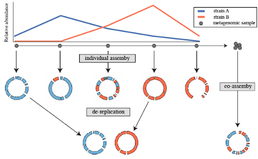 Open image in new tab
Several tools have been designed for the process of de-replication. dRep (Olm et al. 2017) is a software tool designed for the dereplication of genomes in metagenomic datasets. The goal is to retain a representative set of genomes to improve downstream analyses, such as taxonomic profiling and functional annotation.
An typical workflow of how dRep works for dereplication in metagenomics includes:
-
Genome Comparison: dRep uses a pairwise genome comparison approach to assess the similarity between genomes in a given metagenomic dataset.
-
Clustering: Based on the genome similarities, dRep performs clustering to group similar genomes into “genome clusters.” Each cluster represents a group of closely related genomes.
-
Genome Quality Assessment: dRep evaluates the quality of each genome within a cluster. It considers factors such as completeness, contamination, and strain heterogeneity.
-
Genome Selection: Within each genome cluster, dRep selects a representative genome based on user-defined criteria. This representative genome is considered the “dereplicated” version of the cluster.
-
Dereplication Output: The output of dRep includes information about the dereplicated genomes, including their identity, completeness, and contamination. The user can choose a threshold for genome similarity to control the level of dereplication.
Hands On: General list of actions for de-replication
- Create new history
- Assemble each sample separately using your favorite assembler
- Perform a co-assembly to catch low-abundance microbes
- Bin each assembly separately using your favorite binner
- Bin co-assembly using your favorite binner
- Pull the bins from all assemblies together
- Run dRep dereplication ( Galaxy version 3.6.2+galaxy1) on them
- Perform downstream analysis on the de-replicated genome list
Conclusions
In summary, this tutorial shows a step-by-step guide on how to bin metagenomic contigs using various binners, including bin refinement.
It is critical to select the appropriate binning tool for a specific metagenomics study, as different binning methods may have different strengths and limitations depending on the type of metagenomic data being analyzed. By comparing the outcomes of several binning techniques, researchers can increase the precision and accuracy of genome binning.
There are various binning methods available for metagenomic data, including reference-based, clustering-based, hybrid approaches, and machine learning. Each method has its advantages and disadvantages, and the selection of the appropriate method depends on the research question and the characteristics of the data.
Comparing the outcomes of multiple binning methods can help to identify the most accurate and reliable method for a specific study. This can be done by evaluating the quality of the resulting bins in terms of completeness, contamination, and strain heterogeneity, as well as by comparing the composition and functional profiles of the identified genomes.
Overall, by carefully selecting and comparing binning methods, researchers can improve the quality and reliability of genome bins, which can ultimately lead to a better understanding of the functional and ecological roles of microbial communities in various environments.
You've Finished the Tutorial
Key points
Metagenomics binning is a computational approach to grouping together DNA sequences from a mixed microbial sample into metagenome-assembled genomes (MAGs)
The metagenomics binning workflow involves several steps, including preprocessing of raw sequencing data, assembly of sequencing reads into contigs, binning of contigs into MAGs, quality assessment of MAGs, and annotation of functional genes and metabolic pathways in MAGs
The quality and completeness of MAGs can be evaluated using standard metrics, such as completeness, contamination, and genome size
Metagenomics binning can be used to gain insights into the composition, diversity, and functional potential of microbial communities, and can be applied to a range of research areas, such as human health, environmental microbiology, and biotechnology
Frequently Asked Questions
Have questions about this tutorial? Have a look at the available FAQ pages and support channelsUseful literature
Further information, including links to documentation and original publications, regarding the tools, analysis techniques and the interpretation of results described in this tutorial can be found here.
References
- Alneberg, J., B. S. Bjarnason, I. de Bruijn, M. Schirmer, J. Quick et al., 2014 Binning metagenomic contigs by coverage and composition. Nature Methods 11: 1144–1146. 10.1038/nmeth.3103
- Imelfort, M., D. Parks, B. J. Woodcroft, P. Dennis, P. Hugenholtz et al., 2014 GroopM: an automated tool for the recovery of population genomes from related metagenomes. PeerJ 2: e603. 10.7717/peerj.603
- Eren, A. M., Özcan C. Esen, C. Quince, J. H. Vineis, H. G. Morrison et al., 2015 Anvi’o: an advanced analysis and visualization platform for ‘omics data. PeerJ 3: e1319. 10.7717/peerj.1319
- Parks, D. H., M. Imelfort, C. T. Skennerton, P. Hugenholtz, and G. W. Tyson, 2015 CheckM: assessing the quality of microbial genomes recovered from isolates, single cells, and metagenomes. Genome Research 25: 1043–1055. 10.1101/gr.186072.114
- Wu, Y.-W., B. A. Simmons, and S. W. Singer, 2015 MaxBin 2.0: an automated binning algorithm to recover genomes from multiple metagenomic datasets. Bioinformatics 32: 605–607. 10.1093/bioinformatics/btv638
- Lin, H.-H., and Y.-C. Liao, 2016 Accurate binning of metagenomic contigs via automated clustering sequences using information of genomic signatures and marker genes. Scientific Reports 6: 10.1038/srep24175
- Olm, M. R., C. T. Brown, B. Brooks, and J. F. Banfield, 2017 dRep: a tool for fast and accurate genomic comparisons that enables improved genome recovery from metagenomes through de-replication. The ISME journal 11: 2864–2868. 10.1038/ismej.2017.126
- Sieber, C. M. K., A. J. Probst, A. Sharrar, B. C. Thomas, M. Hess et al., 2018 Recovery of genomes from metagenomes via a dereplication, aggregation and scoring strategy. Nature Microbiology 3: 836–843. 10.1038/s41564-018-0171-1
- Uritskiy, G. V., J. DiRuggiero, and J. Taylor, 2018 MetaWRAP—a flexible pipeline for genome-resolved metagenomic data analysis. Microbiome 6: 10.1186/s40168-018-0541-1
- Kang, D. D., F. Li, E. Kirton, A. Thomas, R. Egan et al., 2019 MetaBAT 2: an adaptive binning algorithm for robust and efficient genome reconstruction from metagenome assemblies. PeerJ 7: e7359. 10.7717/peerj.7359
- Nissen, J. N., J. Johansen, R. L. Allesøe, C. K. Sønderby, J. J. A. Armenteros et al., 2021 Improved metagenome binning and assembly using deep variational autoencoders. Nature biotechnology 39: 555–560. 10.1038/s41587-020-00777-4
- Meyer, F., A. Fritz, Z. L. Deng, D. Koslicki, T. R. Lesker et al., 2022 Critical Assessment of Metagenome Interpretation: the second round of challenges. Nature Methods 19: 429–440. 10.1038/s41592-022-01431-4
- Pan, S., C. Zhu, X.-M. Zhao, and L. P. Coelho, 2022 A deep siamese neural network improves metagenome-assembled genomes in microbiome datasets across different environments. Nature Communications 13: 10.1038/s41467-022-29843-y
- Chklovski, A., D. H. Parks, B. J. Woodcroft, and G. W. Tyson, 2023 CheckM2: a rapid, scalable and accurate tool for assessing microbial genome quality using machine learning. Nature methods 20: 1203–1212. 10.1101/2022.07.11.499243
- Mainguy, J., and C. Hoede, 2024 Binette: a fast and accurate bin refinement tool to construct high‐quality Metagenome Assembled Genomes. Journal of Open Source Software 9: 6782. 10.21105/joss.06782
- Wang, Z., R. You, H. Han, W. Liu, F. Sun et al., 2024 Effective binning of metagenomic contigs using contrastive multi‑view representation learning. Nature Communications 15: 10.1038/s41467-023-44290-z
- Author, A., B. Author, and C. Author, 2025 Comprehensive benchmarking of metagenomic binners across diverse environments. Nature Communications 16: 57957. 10.1038/s41467-025-57957-6
Feedback
Did you use this material as an instructor? Feel free to give us feedback on how it went.
Did you use this material as a learner or student? Click the form below to leave feedback.

Citing this Tutorial
- Paul Zierep, Nikos Pechlivanis, Fotis E. Psomopoulos, Vini Salazar, Binning of metagenomic sequencing data (Galaxy Training Materials). https://training.galaxyproject.org/training-material/topics/microbiome/tutorials/metagenomics-binning/tutorial.html Online; accessed TODAY
- Hiltemann, Saskia, Rasche, Helena et al., 2023 Galaxy Training: A Powerful Framework for Teaching! PLOS Computational Biology 10.1371/journal.pcbi.1010752
- Batut et al., 2018 Community-Driven Data Analysis Training for Biology Cell Systems 10.1016/j.cels.2018.05.012
Congratulations on successfully completing this tutorial!@misc{microbiome-metagenomics-binning, author = "Paul Zierep and Nikos Pechlivanis and Fotis E. Psomopoulos and Vini Salazar", title = "Binning of metagenomic sequencing data (Galaxy Training Materials)", year = "", month = "", day = "", url = "\url{https://training.galaxyproject.org/training-material/topics/microbiome/tutorials/metagenomics-binning/tutorial.html}", note = "[Online; accessed TODAY]" } @article{Hiltemann_2023, doi = {10.1371/journal.pcbi.1010752}, url = {https://doi.org/10.1371%2Fjournal.pcbi.1010752}, year = 2023, month = {jan}, publisher = {Public Library of Science ({PLoS})}, volume = {19}, number = {1}, pages = {e1010752}, author = {Saskia Hiltemann and Helena Rasche and Simon Gladman and Hans-Rudolf Hotz and Delphine Larivi{\`{e}}re and Daniel Blankenberg and Pratik D. Jagtap and Thomas Wollmann and Anthony Bretaudeau and Nadia Gou{\'{e}} and Timothy J. Griffin and Coline Royaux and Yvan Le Bras and Subina Mehta and Anna Syme and Frederik Coppens and Bert Droesbeke and Nicola Soranzo and Wendi Bacon and Fotis Psomopoulos and Crist{\'{o}}bal Gallardo-Alba and John Davis and Melanie Christine Föll and Matthias Fahrner and Maria A. Doyle and Beatriz Serrano-Solano and Anne Claire Fouilloux and Peter van Heusden and Wolfgang Maier and Dave Clements and Florian Heyl and Björn Grüning and B{\'{e}}r{\'{e}}nice Batut and}, editor = {Francis Ouellette}, title = {Galaxy Training: A powerful framework for teaching!}, journal = {PLoS Comput Biol} }
You can use Ephemeris's
shed-tools installcommand to install the tools used in this tutorial.shed-tools install [-g GALAXY] [-a API_KEY] -t <(curl https://training.galaxyproject.org/training-material/api/topics/microbiome/tutorials/metagenomics-binning/tutorial.json | jq .admin_install_yaml -r)Alternatively you can copy and paste the following YAML
---
install_tool_dependencies: true
install_repository_dependencies: true
install_resolver_dependencies: true
tools:
- name: bowtie2
  owner: devteam
  revisions: f76cbb84d67f
  tool_panel_section_label: Mapping
  tool_shed_url: https://toolshed.g2.bx.psu.edu/
- name: samtools_sort
  owner: devteam
  revisions: f2f2650aeade
  tool_panel_section_label: SAM/BAM
  tool_shed_url: https://toolshed.g2.bx.psu.edu/
- name: binette
  owner: iuc
  revisions: 37ab2cfedac4
  tool_panel_section_label: Metagenomic Analysis
  tool_shed_url: https://toolshed.g2.bx.psu.edu/
- name: checkm_lineage_wf
  owner: iuc
  revisions: f0107b9f2dc3
  tool_panel_section_label: Metagenomic Analysis
  tool_shed_url: https://toolshed.g2.bx.psu.edu/
- name: concoct
  owner: iuc
  revisions: eae7ee167917
  tool_panel_section_label: Metagenomic Analysis
  tool_shed_url: https://toolshed.g2.bx.psu.edu/
- name: concoct_coverage_table
  owner: iuc
  revisions: fd31cd168efc
  tool_panel_section_label: Metagenomic Analysis
  tool_shed_url: https://toolshed.g2.bx.psu.edu/
- name: concoct_cut_up_fasta
  owner: iuc
  revisions: 4d8bc5dd9e95
  tool_panel_section_label: Metagenomic Analysis
  tool_shed_url: https://toolshed.g2.bx.psu.edu/
- name: concoct_extract_fasta_bins
  owner: iuc
  revisions: 8b1b09fcd8b7
  tool_panel_section_label: Metagenomic Analysis
  tool_shed_url: https://toolshed.g2.bx.psu.edu/
- name: concoct_merge_cut_up_clustering
  owner: iuc
  revisions: 20ccec4a2c38
  tool_panel_section_label: Metagenomic Analysis
  tool_shed_url: https://toolshed.g2.bx.psu.edu/
- name: das_tool
  owner: iuc
  revisions: b048a987dd7d
  tool_panel_section_label: Metagenomic Analysis
  tool_shed_url: https://toolshed.g2.bx.psu.edu/
- name: drep_dereplicate
  owner: iuc
  revisions: f54e7b3da33c
  tool_panel_section_label: Metagenomic Analysis
  tool_shed_url: https://toolshed.g2.bx.psu.edu/
- name: fasta_to_contig2bin
  owner: iuc
  revisions: fb2bed0eb02f
  tool_panel_section_label: Metagenomic Analysis
  tool_shed_url: https://toolshed.g2.bx.psu.edu/
- name: metabat2
  owner: iuc
  revisions: f375b4f6ef57
  tool_panel_section_label: Metagenomic Analysis
  tool_shed_url: https://toolshed.g2.bx.psu.edu/
- name: metabat2_jgi_summarize_bam_contig_depths
  owner: iuc
  revisions: 00e3b4ef7e0c
  tool_panel_section_label: Metagenomic Analysis
  tool_shed_url: https://toolshed.g2.bx.psu.edu/
- name: semibin
  owner: iuc
  revisions: afee33334a63
  tool_panel_section_label: Metagenomic Analysis
  tool_shed_url: https://toolshed.g2.bx.psu.edu/
- name: maxbin2
  owner: mbernt
  revisions: '0917b2d6010d'
  tool_panel_section_label: Metagenomic Analysis
  tool_shed_url: https://toolshed.g2.bx.psu.edu/