Predicting Mutation Impact with Zero-shot Learning using a pretrained DNA LLM
| Author(s) |
|
| Reviewers |
|
OverviewQuestions:
Objectives:
How does zero-shot learning differ from traditional supervised learning, and what advantages does it offer in the context of predicting DNA mutation impacts?
What steps are involved in computing embeddings for DNA sequences using a pre-trained LLM, and how do these embeddings capture the semantic meaning of the sequences?
Why is the L2 distance used as a metric to quantify the impact of mutations, and how does a higher L2 distance indicate a more significant mutation effect?
Requirements:
Explain the concept of zero-shot learning and its application in predicting the impact of DNA mutations using pre-trained large language models (LLMs).
Utilize a pre-trained DNA LLM from Hugging Face to compute embeddings for wild-type and mutated DNA sequences.
Compare the embeddings of wild-type and mutated sequences to quantify the impact of mutations using L2 distance as a metric.
Interpret the results of the L2 distance calculations to determine the significance of mutation effects and discuss potential implications in genomics research.
Develop a script to automate the process of predicting mutation impacts using zero-shot learning, enabling researchers to apply this method to their own datasets efficiently.
- tutorial Hands-on: Introduction to Python
- tutorial Hands-on: Python - Warm-up for statistics and machine learning
- tutorial Hands-on: Foundational Aspects of Machine Learning using Python
- slides Slides: Neural networks using Python
- tutorial Hands-on: Neural networks using Python
- slides Slides: Deep Learning (without Generative Artificial Intelligence) using Python
- tutorial Hands-on: Deep Learning (without Generative Artificial Intelligence) using Python
- tutorial Hands-on: Pretraining a Large Language Model (LLM) from Scratch on DNA Sequences
- tutorial Hands-on: Fine-tuning a LLM for DNA Sequence Classification
Time estimation: 3 hoursLevel: Intermediate IntermediateSupporting Materials:Published: Apr 17, 2025Last modification: May 22, 2025License: Tutorial Content is licensed under Creative Commons Attribution 4.0 International License. The GTN Framework is licensed under MITpurl PURL: https://gxy.io/GTN:T00523version Revision: 4
Best viewed in a Jupyter NotebookThis tutorial is best viewed in a Jupyter notebook! You can load this notebook one of the following ways
Run on the GTN with JupyterLite (in-browser computations)
Launching the notebook in Jupyter in Galaxy
- Instructions to Launch JupyterLab
- Open a Terminal in JupyterLab with File -> New -> Terminal
- Run
wget https://training.galaxyproject.org/training-material/topics/statistics/tutorials/genomic-llm-zeroshot-prediction/statistics-genomic-llm-zeroshot-prediction.ipynb- Select the notebook that appears in the list of files on the left.
Downloading the notebook
- Right click one of these links: Jupyter Notebook (With Solutions), Jupyter Notebook (Without Solutions)
- Save Link As..
Predicting the impact of mutations is a critical task in genomics, as it provides insights into how genetic variations influence biological functions and contribute to diseases. Traditional methods for assessing mutation impact often rely on extensive experimental data or computationally intensive simulations. However, with the advent of large language models (LLMs) and zero-shot learning, we can now predict mutation impacts more efficiently and effectively.
Zero-shot learning is a technique that allows a pre-trained model to make predictions on tasks it wasn’t explicitly trained for, leveraging its existing knowledge. This approach is particularly valuable when labeled data is scarce or when rapid predictions are needed. By using a pre-trained DNA LLM, we can compute embeddings for both wild-type and mutated DNA sequences and compare them to quantify the impact of mutations.
This tutorial focuses on this innovative method, utilizing a pre-trained DNA LLM available on Hugging Face to assess the impact of mutations. This approach opens new avenues for bioinformatics research, particularly in genomics and personalized medicine, by enabling researchers to gain insights into the functional impact of DNA mutations efficiently.
Building upon this foundation, our new tutorial focuses on predicting the impact of mutations using zero-shot learning with a pre-trained DNA LLM. Zero-shot learning allows us to utilize the pre-trained model directly, without additional training, to make predictions on new, unseen tasks. Specifically, we will use a pre-trained model available on Hugging Face, designed for DNA sequences, to assess the impact of mutations.
We will use Mistral-DNA-v1-17M-hg38, a mixed model that was pre-trained on the entire Human Genome. It contains approximately 17 million parameters and was trained using the Human Genome assembly GRCh38 on sequences of 10,000 bases (10K):
model_name="RaphaelMourad/Mistral-DNA-v1-17M-hg38"
AgendaIn this tutorial, we will cover:
Prepare resources
Install dependencies
The first step is to install the required dependencies:
!pip install Bio==1.7.1
!pip install transformers -U
Import Python libraries
Let’s now import them.
import os

import matplotlib.pyplot as plt
import numpy as np
import scipy as sp
import torch
import tensorflow as tf
import gzip
from Bio import SeqIO
from transformers import (
  AutoConfig,
  AutoModelForCausalLM,
  AutoTokenizer,
  EarlyStoppingCallback,
  Trainer,
  TrainingArguments,
)
Comment: VersionsThis tutorial has been tested with following versions:
transformers= 4.48.3You can check the versions with:
transformers.__version__
Check and configure available resources
We select the appropriate device (CUDA-enabled GPU if available) for running PyTorch operations
torch.device('cuda' if torch.cuda.is_available() else 'cpu')
Let’s check the GPU usage and RAM:
!nvidia-smi
Let’s configure PyTorch and the CUDA environment – software and hardware ecosystem provided by NVIDIA to enable parallel computing on GPU – to optimize GPU memory usage and performance:
-
Enables CuDNN benchmarking in PyTorch:
torch.backends.cudnn.benchmark=True -
Set an environment variable that configures how PyTorch manages CUDA memory allocations
os.environ["PYTORCH_CUDA_ALLOC_CONF"] = "max_split_size_mb:32"
Tokenizing DNA Sequences
We now set up the tokenizer to convert raw DNA sequences into a format that the model can process, enabling it to understand and analyze the sequences effectively:
tokenizer = transformers.AutoTokenizer.from_pretrained(
    model_name,
    use_fast=True,
    trust_remote_code=True,
)
QuestionWhat do the parameters?
use_fast=True?trust_remote_code=True?
use_fast=True: Enables the use of a fast tokenizer implementation, which is optimized for speed and efficiency. This is particularly useful when working with large datasets or when performance is a priority.trust_remote_code=True: Allows the tokenizer to execute custom code from the model repository. This may be necessary for certain architectures or preprocessing steps that require additional functionality.
Load and Configure the Pre-trained Model
We will now load the pre-trained DNA large language model (LLM) and configure it for our specific task of predicting the impact of DNA mutations.
model=transformers.AutoModelForCausalLM.from_pretrained(
    model_name,
)
We would like to ensure that the model correctly handles padding tokens, which are used to standardize the length of sequences within a batch:
model.config.pad_token_id = tokenizer.pad_token_id
Aligning the padding token ID between the model and tokenizer is crucial for maintaining consistency during training and inference.
Let’s look at the model:
model
MixtralForCausalLM(
  (model): MixtralModel(
    (embed_tokens): Embedding(4096, 256)
    (layers): ModuleList(
      (0-7): 8 x MixtralDecoderLayer(
        (self_attn): MixtralAttention(
          (q_proj): Linear(in_features=256, out_features=256, bias=False)
          (k_proj): Linear(in_features=256, out_features=256, bias=False)
          (v_proj): Linear(in_features=256, out_features=256, bias=False)
          (o_proj): Linear(in_features=256, out_features=256, bias=False)
        )
        (block_sparse_moe): MixtralSparseMoeBlock(
          (gate): Linear(in_features=256, out_features=8, bias=False)
          (experts): ModuleList(
            (0-7): 8 x MixtralBlockSparseTop2MLP(
              (w1): Linear(in_features=256, out_features=256, bias=False)
              (w2): Linear(in_features=256, out_features=256, bias=False)
              (w3): Linear(in_features=256, out_features=256, bias=False)
              (act_fn): SiLU()
            )
          )
        )
        (input_layernorm): MixtralRMSNorm((256,), eps=1e-05)
        (post_attention_layernorm): MixtralRMSNorm((256,), eps=1e-05)
      )
    )
    (norm): MixtralRMSNorm((256,), eps=1e-05)
    (rotary_emb): MixtralRotaryEmbedding()
  )
  (lm_head): Linear(in_features=256, out_features=4096, bias=False)
)
QuestionWhat do the parameters?
- How does the vocabulary size of 4,096 relate to k-mers in DNA sequences?
- What is the role of the embedding layer in
MixtralForCausalLM?- How many layers does the
MixtralForCausalLMmodel have, and what is their purpose?- What components make up the self-attention mechanism in MixtralAttention?
- How does the Mixture of Experts (MoE) mechanism reduce computational load?
- Why is layer normalization important in
MixtralForCausalLM?- What advantage do rotary embeddings offer in understanding DNA sequences?
- The vocabulary size corresponds to the number of unique “words” or k-mers (subsequences of DNA) the model can recognize, similar to using k-mers of size six, enhanced by byte-pair encoding for more nuanced patterns.
- The embedding layer converts DNA sequences into numerical vectors, enabling the model to process and analyze them.
- The model has 8 layers, each containing a
MixtralDecoderLayer. These layers process the embedded input sequences through a series of transformations, including self-attention and mixture of experts, to capture complex patterns in the data.- The self-attention mechanism includes query, key, value, and output projections, which weigh the importance of different tokens in the sequence.
- MoE activates only a subset of parameters during each forward pass, using a routing mechanism to direct sequences to specific experts.
- Layer normalization stabilizes and accelerates training by ensuring consistent scaling of inputs to the attention mechanism and subsequent layers.
- Rotary embeddings enhance the model’s understanding of positional information, providing a more nuanced representation of sequence order compared to traditional methods.
QuestionFor a DNA sequence “ACGTAGCATCGGATCTATCTATCGACACTTGGTTATCGATCTACGAGCATCTCGTTAGC”
- How can we get the hidden states?
- How can we compute mean of the hidden states accross the sequence length dimension?
- What is the shape of the output?
- What does the mean of the hidden states accross the sequence length dimension represent?
Let’s start by defining the DNA sequence:
dna = "ACGTAGCATCGGATCTATCTATCGACACTTGGTTATCGATCTACGAGCATCTCGTTAGC"
- To get the hidden state:
Tokenize the DNA sequence using the tokenizer
tokenized_dna = tokenizer(dna, return_tensors = "pt")Extract the tensor containing the token IDs from the tokenized output
inputs = tokenized_dna["input_ids"]Pass the tokenized input through the model.
model_outputs = model(inputs)Extract the hidden states from the model’s output.
hidden_states = model_outputs[0].detach()To compute mean of the hidden states accross the sequence length dimension:
embedding_mean = torch.mean(hidden_states[0], dim=0)The shape is 4,096, the number of possible tokens
- It represents the average embedding of the DNA sequence. This fixed-size representation can be used for various downstream tasks, such as classification, clustering, or similarity comparisons.
Compare the effect of mutations with or without amino acid modification
Let’s look at the portion of the Cystic fibrosis transmembrane conductance regulator (CFTR) gene where a mutation responsible of the Cystic fibrosis appears.
In this portion, we can observe several cases:
| Cases | Sequences |
|---|---|
| Wild-type without any mutation | ATTAAAGAAAATATCATCTTTGGTGTTTCCTAT |
| Mutation ATT to ATA | ATAAAAGAAAATATCATCTTTGGTGTTTCCTAT |
| Deletion of TCT codon | ATTAAAGAAAATATCA—TTGGTGTTTCCTAT |
In the second case, the amino acid does not change (silent mutation). In the last case, an amino acid is removed. Let’s look if the mutation and the deletion have the same distance to the wild-type when computing using the DNA embedding.
First, we define the sequences:
dna_wt= "ATTAAAGAAAATATCATCTTTGGTGTTTCCTAT"
dna_mut="ATAAAAGAAAATATCATCTTTGGTGTTTCCTAT"
dna_del="ATTAAAGAAAATATCATTGGTGTTTCCTAT"
Let’s compute the hidden states for all DNA sequences:
tokenized_dna = tokenizer(
  [dna_wt, dna_mut, dna_del],
  return_tensors="pt",
  padding=True,
)
inputs_seqs = tokenized_dna["input_ids"]
model_outputs = model(inputs_seqs)
hidden_states = model_outputs[0].detach()
We now compute the maximum of the hidden states accross the sequence length dimension:
embedding_max = torch.max(hidden_states, dim=1)[0]
To compare the effects of silent mutation and amino acid deletion, we will compute the distance between the wild-type embeddings and the mutation / deletion embedding using the L2 (Euclidean) distance
The L2 distance, also known as the Euclidean distance, is a measure of the straight-line distance between two points in Euclidean space. It is commonly used to quantify the difference between two vectors, such as embeddings in machine learning.
For two vectors \(a\) and \(b\) in an \(n\)-dimensional space, where \(a=[a\_{1},a\_{2},...,a\_{n}]\) and \(b=[b\_{1},b\_{2},...,b\_{n}]\), the L2 distance is calculated as:
\(L2 = \sqrt{\sum_{i} (a_{i}-b_{i})^{2}\)
wt_mut_L2 = torch.norm(embedding_max[0] - embedding_max[1])
print(wt_mut_L2)
wt_del_L2 = torch.norm(embedding_max[0] - embedding_max[2])
print(wt_del_L2)
tensor(27.4657)
tensor(145.7797)
Question
- Is it the silent mutation or the amino acid deletion that have the lowest L2 distance to the wild-type?
- How to interpret the result?
- The silent mutation has a lower L2 distance to the wild-type compared to the mutation with amino acid deletion.
- A smaller L2 distance indicates that the sequences are more similar, while a larger distance suggests greater dissimilarity.
Compare effects of SNPs in exons and introns
Single Nucleotide Polymorphisms (SNPs) are the most common type of genetic variation, involving a change in a single nucleotide within a DNA sequence. These variations can occur in different regions of the genome, including exons (the coding regions of genes) and introns (the non-coding regions within genes). Understanding the impact of SNPs in these regions is crucial for assessing their role in genetic disorders, phenotypic traits, and overall genome function.
We will now leverage the pre-trained DNA language model to compare the effects of SNPs in exons and introns. By utilizing embeddings generated from DNA sequences, we can quantify the impact of these variations and gain insights into their functional consequences.
Load sequences
To begin our analysis, we need to load the sequence data, which includes sequences with Single Nucleotide Polymorphisms (SNPs) and their corresponding reference sequences (wild-type) without SNPs. These sequences are derived from both introns and exons and are stored in compressed FASTA format on GitHub:
| Wild-type (without SNPs) | Mutated (with SNP) | |
|---|---|---|
| Intron | SNPintron_ref_201b.fasta.gz |
SNPintron_alt_201b.fasta.gz |
| Exon | SNPexon_ref_201b.fasta.gz |
SNPexon_alt_201b.fasta.gz |
baseurl = "https://github.com/raphaelmourad/Mistral-DNA/raw/refs/head/master/data/SNP/"
win=201
exon_wt_snp_fp = f"{ baseurl }/SNPexon_ref_{ win }b.fasta.gz"
exon_mut_snp_fp = f"{ baseurl }/SNPexon_alt_{ win }b.fasta.gz"
intron_wt_snp_fp = f"{ baseurl }/SNPintron_ref_{ win }b.fasta.gz"
intron_mut_snp_fp = f"{ baseurl }/SNPintron_alt_{ win }b.fasta.gz"
We need to get files and read the sequences from them:
import requests
def downloadReadFastaFile(fasta_file):
  response = requests.get(fasta_file)
  # Check if the request was successful
  if response.status_code == 200:
      # Open a local file in binary write mode and save the content
      with open('file.gz', 'wb') as file:
          file.write(response.content)
      print("File downloaded successfully.")
  else:
      print(f"Failed to download file. HTTP Status code: {response.status_code}")
  # Read the file
  seql_list=[]
  with gzip.open("file.gz", "rt") as handle:
      for record in SeqIO.parse(handle, "fasta"):
          seqj=str(record.seq)
          seql_list.append(seqj)
  return seql_list

exon_wt_seqs = downloadReadFastaFile(exon_wt_snp_fp)
exon_mut_seqs = downloadReadFastaFile(exon_mut_snp_fp)
intron_wt_seqs = downloadReadFastaFile(intron_wt_snp_fp)
intron_mut_seqs = downloadReadFastaFile(intron_mut_snp_fp)
Question
- How many sequences are in the data?
- How long are the sequences?
len( exon_wt_seqs ) , len(exon_mut_seqs) , len(intron_wt_seqs) , len( intron_mut_seqs )
(10000, 10000, 10000, 10000)- the sequences are 201 nucleotides long.
We will keep only the 100 first sequences:
kseq = 100
exon_wt_seqs = exon_wt_seqs[0:kseq]
exon_mut_seqs = exon_mut_seqs[0:kseq]
intron_wt_seqs = intron_wt_seqs[0:kseq]
intron_mut_seqs = intron_mut_seqs[0:kseq]
QuestionHow many differences (SNPs) between reference and alternative sequences are there for first exon sequence?
n_diff = 0
for i in range( len( exon_wt_seqs[0] ) ) :
    n_diff += exon_mut_seqs[0][i] == exon_wt_seqs[0][i]
print(n_diff)
Compute effect of SNPs
To compute the effect of SNPs, we need :
- Compute the embdedding of DNA sequences
  def computeEmbedding(seqs):
    tokenized_dna = tokenizer(
      seqs,
      return_tensors="pt",
      padding=True,
    )
    inputs_seqs = tokenized_dna["input_ids"]
    hidden_states = model(inputs_seqs)[0].detach().cpu()
    return torch.max(hidden_states, dim=1)[0]
- Compute the L2 distance between reference (without SNP) and alternative (with SNP):
  def computeMutationEffect(wt_seqs, mut_seqs):
    wt_embedding = computeEmbedding(wt_seqs)
    mut_embedding = computeEmbedding(mut_seqs)
    return torch.norm(mut_embedding - wt_embedding, dim=1)
exon_SNP_distL2 = computeMutationEffect(exon_wt_seqs, exon_mut_seqs)
intron_SNP_distL2 = computeMutationEffect(intron_wt_seqs,intron_mut_seqs)
QuestionWhat are the dimensions of
exon_SNP_distL2andintron_SNP_distL2?10,000 each: one value per pair of wt/mutated sequence
Compare SNPs effects between introns and exons
We can now quantify the impact of SNPs and determine if the differences are statistically significant.
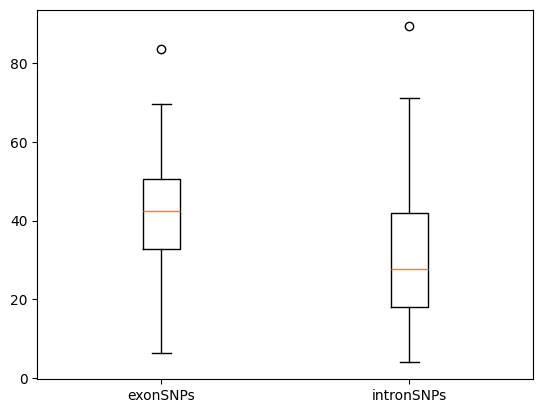
To visualize the predicted effects of SNPs, we can use a boxplot to compare the L2 distances for SNPs in exons and introns. The L2 distance serves as a metric for the impact of mutations, with higher distances indicating a more significant effect.
Boxplot of predicted SNP effects
SNPs_distL2 = {"exons": exon_SNP_distL2, "introns": intron_SNP_distL2}

fig, ax = plt.subplots()
ax.boxplot(SNPs_distL2.values())
ax.set_xticklabels(SNPs_distL2.keys())
Question
What can we conclude from the boxplot?
From the plot, we observe that the L2 distance is generally higher for SNPs in exons compared to those in introns. This suggests that SNPs in exons have a stronger predicted effect, which aligns with their role in coding regions of genes.
To determine if the observed differences in L2 distances are statistically significant, we can perform hypothesis tests to compare the distributions:
-
T-test:
sp.stats.ttest_ind(exon_SNP_distL2, intron_SNP_distL2)QuestionWhat can we conclude from the t-test?
The t-test yields a p-value of approximately \(7.56 \cdot 10^{−7}\), indicating a statistically significant difference between the L2 distances of SNPs in exons and introns.
-
Wilcoxon rank-sum test:
sp.stats.wilcoxon(exon_SNP_distL2, intron_SNP_distL2)QuestionWhat can we conclude from the Wilcoxon test?
The Wilcoxon rank-sum test also shows a significant p-value of approximately \(2.87 \cdot 10^{−6}\), confirming that the distributions are significantly different.
The analysis demonstrates that SNPs in exons have a more substantial impact on the sequence embeddings compared to SNPs in introns, as evidenced by higher L2 distances. This finding is statistically significant, highlighting the importance of exonic SNPs in potentially altering gene function and expression. By understanding these differences, researchers can gain insights into the functional consequences of genetic variations in different genomic regions.
Conclusion
Throughout this tutorial, we explored a comprehensive workflow for analyzing DNA sequences and assessing the impact of mutations using a pre-trained DNA language model. We began by tokenizing DNA sequences, converting them into numerical representations that the model could process and analyze effectively. Following this, we loaded and configured a pre-trained model to handle these sequences, ensuring seamless integration with the tokenizer. We then delved into comparing the effects of mutations, both with and without amino acid modifications, showcasing the model’s ability to discern subtle differences in sequence impacts. Furthermore, we focused on analyzing the effects of Single Nucleotide Polymorphisms (SNPs) in exons and introns. By loading the relevant sequences, computing the L2 distances between embeddings of wild-type and mutated sequences, and visualizing the results, we quantified and compared the impact of SNPs in these regions. Our analysis revealed that SNPs in exons generally have a more significant impact than those in introns, a finding supported by statistical tests. This tutorial underscores the power of pre-trained models in bioinformatics, offering valuable insights into the functional consequences of genetic variations and paving the way for further research in genomics.
You've Finished the Tutorial
Key points
Pre-trained DNA language models are powerful tools for analyzing genetic sequences, enabling efficient and accurate assessment of mutation impacts without extensive computational resources.
SNPs in exons generally have a more significant impact on gene function compared to those in introns, highlighting the importance of focusing on coding regions for understanding genetic variations.
Utilizing embeddings to quantify the effects of mutations provides a robust method for comparing sequence variations, offering insights into the functional consequences of SNPs and other genetic modifications.
Employing statistical tests, such as t-tests and Wilcoxon rank-sum tests, is crucial for validating observed differences in genetic data, ensuring that findings are supported by empirical evidence.
Frequently Asked Questions
Have questions about this tutorial? Have a look at the available FAQ pages and support channelsFeedback
Did you use this material as an instructor? Feel free to give us feedback on how it went.
Did you use this material as a learner or student? Click the form below to leave feedback.

Citing this Tutorial
- Raphael Mourad, Bérénice Batut, Predicting Mutation Impact with Zero-shot Learning using a pretrained DNA LLM (Galaxy Training Materials). https://training.galaxyproject.org/training-material/topics/statistics/tutorials/genomic-llm-zeroshot-prediction/tutorial.html Online; accessed TODAY
- Hiltemann, Saskia, Rasche, Helena et al., 2023 Galaxy Training: A Powerful Framework for Teaching! PLOS Computational Biology 10.1371/journal.pcbi.1010752
- Batut et al., 2018 Community-Driven Data Analysis Training for Biology Cell Systems 10.1016/j.cels.2018.05.012
Congratulations on successfully completing this tutorial!@misc{statistics-genomic-llm-zeroshot-prediction, author = "Raphael Mourad and Bérénice Batut", title = "Predicting Mutation Impact with Zero-shot Learning using a pretrained DNA LLM (Galaxy Training Materials)", year = "", month = "", day = "", url = "\url{https://training.galaxyproject.org/training-material/topics/statistics/tutorials/genomic-llm-zeroshot-prediction/tutorial.html}", note = "[Online; accessed TODAY]" } @article{Hiltemann_2023, doi = {10.1371/journal.pcbi.1010752}, url = {https://doi.org/10.1371%2Fjournal.pcbi.1010752}, year = 2023, month = {jan}, publisher = {Public Library of Science ({PLoS})}, volume = {19}, number = {1}, pages = {e1010752}, author = {Saskia Hiltemann and Helena Rasche and Simon Gladman and Hans-Rudolf Hotz and Delphine Larivi{\`{e}}re and Daniel Blankenberg and Pratik D. Jagtap and Thomas Wollmann and Anthony Bretaudeau and Nadia Gou{\'{e}} and Timothy J. Griffin and Coline Royaux and Yvan Le Bras and Subina Mehta and Anna Syme and Frederik Coppens and Bert Droesbeke and Nicola Soranzo and Wendi Bacon and Fotis Psomopoulos and Crist{\'{o}}bal Gallardo-Alba and John Davis and Melanie Christine Föll and Matthias Fahrner and Maria A. Doyle and Beatriz Serrano-Solano and Anne Claire Fouilloux and Peter van Heusden and Wolfgang Maier and Dave Clements and Florian Heyl and Björn Grüning and B{\'{e}}r{\'{e}}nice Batut and}, editor = {Francis Ouellette}, title = {Galaxy Training: A powerful framework for teaching!}, journal = {PLoS Comput Biol} }