Identification of the micro-organisms in a beer using Nanopore sequencing
| Author(s) |
|
| Reviewers |
|
OverviewQuestions:
Objectives:
How can yeast strains in a beer sample be identified?
How can we process metagenomic data sequenced using Nanopore?
Requirements:
Inspect metagenomics data
Run metagenomics tools
Identify yeast species contained in a sequenced beer sample using DNA
Visualize the microbiome community of a beer sample
Time estimation: 1 hourLevel: Introductory IntroductorySupporting Materials:Published: Sep 29, 2022Last modification: Nov 29, 2024License: Tutorial Content is licensed under Creative Commons Attribution 4.0 International License. The GTN Framework is licensed under MITpurl PURL: https://gxy.io/GTN:T00384rating Rating: 4.8 (0 recent ratings, 5 all time)version Revision: 5
What is a microbiome? It is a collection of small living creatures. These small creatures are called micro-organisms and they are everywhere. In our gut, in the soil, on vending machines, and even inside the beer. Most of these micro-organisms are actually very good for us, but some can make us very ill.
Micro-organisms come in different shapes and sizes, but they have the same components. One crucial component is the DNA, the blueprint of life. The DNA encodes the shape and size and many other characteristics unique to a species. Because DNA is so species-specific, reading the DNA can be used to identify what kind of micro-organism the it is from. Therefore, within a metagenomic specimen, e.g. a sample form soil, gut, or beer, one can identify what kind of species are inside the sample.
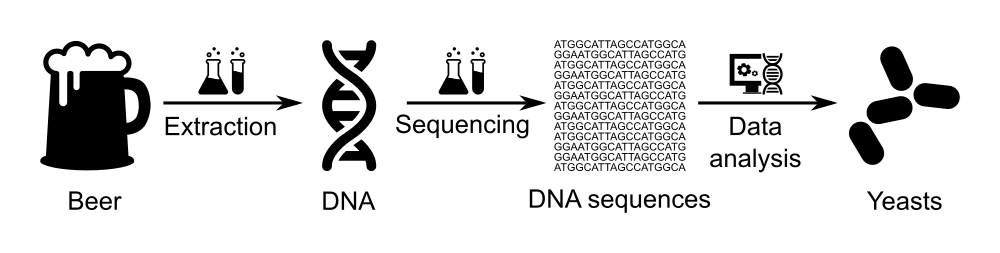
In this tutorial, we will use data of beer microbiome generated via the BeerDEcoded project.
The BeerDEcoded Project is a series of workshops organized with and for schools as well as the general audience, aiming to introduce biology and genomic science. People learn in an interactive way about DNA, sequencing technologies, bioinformatics, open science, how these technologies and concepts are applied and how they are impacting their daily life.
Beer is alive and contains many microorganisms. It can be found in many places and there are many of them. It is a fun media to bring the people to the contact of molecular biology, data-analysis, and open science.
A BeerDEcoded workshop includes the following steps:
- Extract yeasts and their DNA from beer bottle,
- Sequence the extracted DNA using a MinION sequencer to obtain the sequence of bases/nucleotides (A, T, C and G) for each DNA fragment in the sample,
- Analyze the sequenced data in order to know which organisms this DNA is from
Comment: Beer microbiomeBeer is alive! It contains microorganisms, in particular yeasts.
Indeed, grain and water create a sugary liquid (called wort). The beer brewer adds yeasts to it. By eating the sugar, yeast creates alcohol, and other compounds (esters, phenols, etc.) that give beer its particular flavor.
Yeasts are microorganisms, more precisely unicellular fungi. The majority of beers use a yeast genus called Saccharomyces, which in Greek means “sugar fungus”. Within that genus, two specific species of Saccharomyces are the most commonly used:
- Saccharomyces cerevisiae: a top-fermenting (i.e. yeast which rise up to the top of the beer as it metabolizes sugars, delivering alcohol as a by-product), ale yeast responsible for a huge range of beer styles like witbiers, stouts, ambers, tripels, saisons, IPAs, and many more. It is most likely the yeast that the early brewers were inadvertently brewing with over 3,000 years ago.
- Saccharomyces pastorianus: a bottom-fermenting (i.e. it sits on the bottom of the tank as it ferments) lager yeast, responsible for beer styles like Pilsners, lagers, märzens, bocks, and more. This yeast was originally found, and cultivated, by Bavarian brewers a little over 200 years ago. It is the most commonly used yeast in terms of the raw amount of beer produced around the world.
Since yeast is all around us, we can actually brew spontaneously fermented beer by using wild yeasts and souring microbiota floating through the air.
During one BeerDEcoded workshop, we extracted yeasts out of a bottle of Chimay. We then extracted the DNA of these yeasts and sequenced it using a MinION to obtain the DNA sequences. Now, we would like to identify the yeast species sequenced there, and thereby outline the diversity of microorganisms (the microbiome community) in the beer sample.
To get this information, we need to process the sequenced data in a few steps:
- Check the quality of the data
- Assign a taxonomic label, i.e. assign ‘species’ to each sequence
- Visualize the distribution of the different species
This type of data analysis requires running several bioinformatics tools and usually requires a computer science background. Galaxy is an open-source platform for data analysis that enables anyone to use bioinformatics tools through its graphical web interface, accessible via any Web browser.
So, in this tutorial, we will use Galaxy to extract and visualize the community of yeasts from a bottle of beer.
AgendaIn this tutorial, we will cover:
Prepare Galaxy and data
First of all, this tutorial will get you hands on with some basic Galaxy tasks, including creating a history and importing data.
Get familiar with Galaxy
Hands On: Open Galaxy
- Open your favorite browser (Works on Chrome, Firefox, Safari but not Internet Explorer!)
Create a Galaxy account if you do not have one
To create an account at any public Galaxy instance, choose your server from the available list of Galaxy Platforms.
There are several UseGalaxy servers:
UseGalaxy.fr (FR)
UseGalaxy.ca (CA)
UseGalaxy.org (US)
UseGalaxy.eu (EU)
UseGalaxy.org.au (AU)
Click on “Login or Register” in the masthead on the server.
On the login page, find the Register here link and click on it.
Fill in the the registration form, then click on Create.
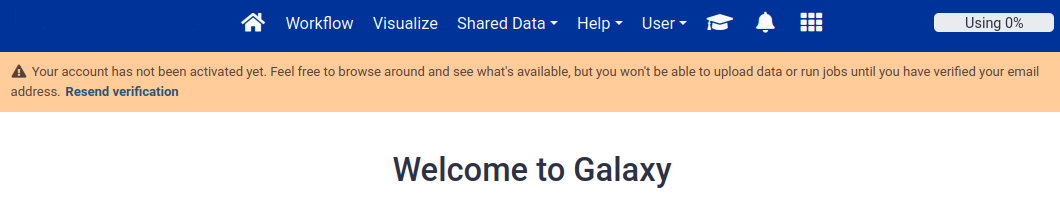
Your account should now get created, but will remain inactive until you verify the email address you provided in the registration form.
Check for a Confirmation Email in the email you used for account creation.
Missing? Check your Trash and Spam folders.
Click on the Email confirmation link to fully activate your account.
galaxy-info Delivery of the confimation email is blocked by your email provider or you mistyped the email address in the registration form?
Please do not register again, but follow the instructions to change the email address registered with your account! The confirmation email will be resent to your new address once you have changed it.
Trouble logging in later? Account email addresses and public names are caSe-sensiTive. Check your activation email for formats.
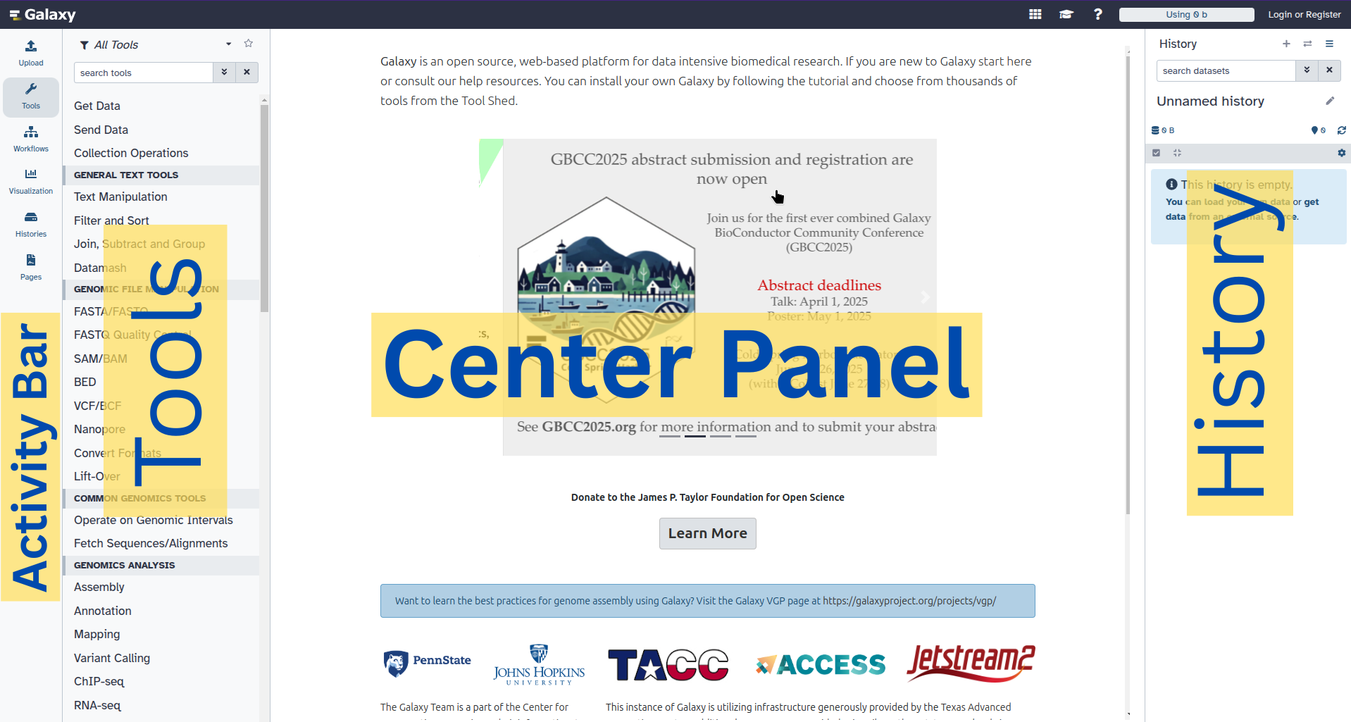
The Galaxy homepage is divided into three panels:
- Tools on the left
- Viewing panel in the middle
- History of analysis and files on the right
 Open image in new tab
The first time you use Galaxy, there will be no files in your history panel.
Any analysis should get its own Galaxy history. So let’s start by creating a new one:
Hands On: Prepare the Galaxy history
Create a new history for this analysis
To create a new history simply click the new-history icon at the top of the history panel:
Rename the history
- Click on galaxy-pencil (Edit) next to the history name (which by default is “Unnamed history”)
- Type the new name
- Click on Save
- To cancel renaming, click the galaxy-undo “Cancel” button
If you do not have the galaxy-pencil (Edit) next to the history name (which can be the case if you are using an older version of Galaxy) do the following:
- Click on Unnamed history (or the current name of the history) (Click to rename history) at the top of your history panel
- Type the new name
- Press Enter

Get data
Before we can begin any Galaxy analysis, we need to upload the input data: FASTQ files
Hands On: Upload your dataset
Import the sequenced data including fastq in the name
Option 1 video: Your own local data using Upload Data (recommended for 1-10 datasets).
- Click on Upload Data on the top of the left panel
- Click on Choose local file and select the files or drop the files in the Drop files here part
- Click on Start
- Click on Close
Option 2: From Zenodo, an external server, via URL
https://zenodo.org/record/7093173/files/ABJ044_c38189e89895cdde6770a18635db438c8a00641b.fastq
- Copy the link location
Click galaxy-upload Upload at the top of the activity panel
- Select galaxy-wf-edit Paste/Fetch Data
Paste the link(s) into the text field
Press Start
- Close the window
Your uploaded file is now in your current history. When the file is fully uploaded to Galaxy, it will turn green. But, what is this file?
Click on the galaxy-eye (eye) icon next to the dataset name to look at the file contents.

The contents of the file will be displayed in the central Galaxy panel.
This file contains the sequences, also called reads, of DNA, i.e. succession of nucleotides, for all fragments from the yeasts in the beer, in FASTQ format.
Although it looks complicated (and maybe it is), the FASTQ format is easy to understand with a little decoding. Each read, representing a fragment of DNA, is encoded by 4 lines:
Line Description 1 Always begins with @followed by the information about the read2 The actual nucleic sequence 3 Always begins with a +and contains sometimes the same info in line 14 Has a string of characters which represent the quality scores associated with each base of the nucleic sequence; must have the same number of characters as line 2 So for example, the first sequence in our file is:
@03dd2268-71ef-4635-8bce-a42a0439ba9a runid=8711537cc800b6622b9d76d9483ecb373c6544e5 read=252 ch=179 start_time=2019-12-08T11:54:28Z flow_cell_id=FAL10820 protocol_group_id=la_trappe sample_id=08_12_2019
AGTAAGTAGCGAACCGGTTTCGTTTGGGTGTTTAACCGTTTTCGCATTTATCGTGAAACGCTTTCGCGTTTTCGTGCGGAAGGCGCTTCACCCAGGGCCTCTCATGCTTTGTCTTCCTGTTTATTCAGGATCGCCCAAAGCGAGAATCATACCACTAGACCACACGCCCGAATTATTGTTGCGTTAATAAGAAAAGCAAATATTTAAGATAGGAAGTGATTAAAGGGAATCTTCTACCAACAATATCCATTCAAATTCAGGCA
+
$'())#$$%#$%%'-$&$%'%#$%('+;<>>>18.?ACLJM7E:CFIMK<=@0/.4<9<&$007:,3<IIN<3%+&$(+#$%'$#$.2@401/5=49IEE=CH.20355>-@AC@:B?7;=C4419)*$$46211075.$%..#,529,''=CFF@:<?9B522.(&%%(9:3E99<BIL?:>RB--**5,3(/.-8B>F@@=?,9'36;:87+/19BAD@=8*''&''7752'$%&,5)AM<99$%;EE;BD:=9<@=9+%$
It means that the fragment named
@03dd2268-71ef-4635-8bce-a42a0439ba9a(ID given in line1) corresponds to:
- the DNA sequence
AGTAAGTAGCGAACCGGTTTCGTTTGGGTGTTTAACCGTTTTCGCATTTATCGTGAAACGCTTTCGCGTTTTCGTGCGGAAGGCGCTTCACCCAGGGCCTCTCATGCTTTGTCTTCCTGTTTATTCAGGATCGCCCAAAGCGAGAATCATACCACTAGACCACACGCCCGAATTATTGTTGCGTTAATAAGAAAAGCAAATATTTAAGATAGGAAGTGATTAAAGGGAATCTTCTACCAACAATATCCATTCAAATTCAGGCA(line2)- this sequence has been sequenced with a quality
$'())#$$%#$%%'-$&$%'%#$%('+;<>>>18.?ACLJM7E:CFIMK<=@0/.4<9<&$007:,3<IIN<3%+&$(+#$%'$#$.2@401/5=49IEE=CH.20355>-@AC@:B?7;=C4419)*$$46211075.$%..#,529,''=CFF@:<?9B522.(&%%(9:3E99<BIL?:>RB--**5,3(/.-8B>F@@=?,9'36;:87+/19BAD@=8*''&''7752'$%&,5)AM<99$%;EE;BD:=9<@=9+%$(line 4).But what does this quality score mean?
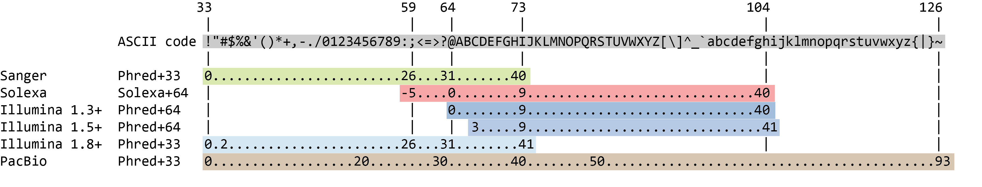
The quality score for each sequence is a string of characters, one for each base of the nucleotide sequence, used to characterize the probability of misidentification of each base. The score is encoded using the ASCII character table (with some historical differences):
So there is an ASCII character associated with each nucleotide, representing its Phred quality score, the probability of an incorrect base call:
Phred Quality Score Probability of incorrect base call Base call accuracy 10 1 in 10 90% 20 1 in 100 99% 30 1 in 1000 99.9% 40 1 in 10,000 99.99% 50 1 in 100,000 99.999% 60 1 in 1,000,000 99.9999%
Data quality
Assess data quality
Before starting to work on our data, it is necessary to assess its quality. This is an essential step if we aim to obtain a meaningful downstream analysis.
FastQC is one of the most widely used tools to check the quality of data generated by High Throughput Sequencing (HTS) technologies.
Hands On: Quality check
- FASTQC ( Galaxy version 0.73+galaxy0) with the following parameters
- param-file “Raw read data from your current history”:
Reads- Inspect the generated HTML file
QuestionGiven the Basic Statistics table on the top of the page:
- How many sequences are in the FASTQ file?
- How long are the sequences?
- There are 1876 sequences.
- The sequences range from 130 nucleotides to 2327 nucleotides. Not all sequences have then the same length.
FastQC provides information on various parameters, such as the range of quality values across all bases at each position:
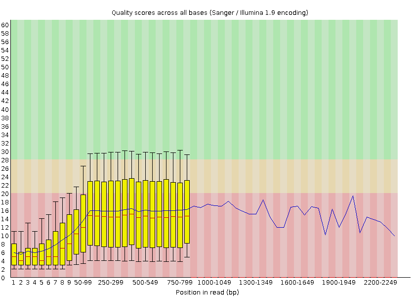 Open image in new tab
We can see that the quality of our sequencing data grows after the first few bases, stays around a score of 18 and then decreases again at the end of the sequences. MinION and Oxford Nanopore Technologies (ONT) are known to have a higher error rate compared to other sequencing techniques and platforms (Delahaye and Nicolas 2021).
For more detailed information about the other plots in the FASTQC report, check out our dedicated tutorial.
Improve the dataset quality
In order to improve the quality of our data, we will use two tools:
- porechop (Wick 2017) to remove adapters that were added for sequencing and chimera (contaminant)
- fastp (Chen et al. 2018) to filter sequences with low quality scores (below 10)
Hands On: Improve the dataset quality
- Porechop ( Galaxy version 0.2.4+galaxy0) with the following parameters:
- param-file “Input FASTA/FASTQ”:
Reads- “Output format for the reads”:
fastq- fastp ( Galaxy version 0.23.2+galaxy0) with the following parameters:
- “Single-end or paired reads”:
Single-end
- param-file “Input 1”: output of Porechop
- In “Adapter Trimming Options”:
- “Disable adapter trimming”:
Yes- In “Filter Options”:
- In “Quality filtering options”:
- “Qualified quality phred”:
10- In “Read Modification Options”:
- “PolyG tail trimming”:
Disable polyG tail trimming- Inspect the HTML report of fastp to see how the quality has been improved
Question
- How many sequences are there before filtering? Is it the same number as in FASTQC report?
- How many sequences are there after filtering? How many sequences have then been removed by filtering?
- What is the mean length before filtering? And after filtering?
- There are 1,869 reads before filtering. The number is lower than in the FASTQC report. Some reads may have been discarded via Porechop
- There are 1,350 reads after filtering. So the filtering step has removed \(1869-1350 = 519\) sequences.
- The mean length is 314 nucleotide before filtering and 316bp after filtering.
Assign taxonomic classification
One of the main aims in microbiome data analysis is to identify the organisms sequenced. For that we try to identify the taxon to which each individual read belong.
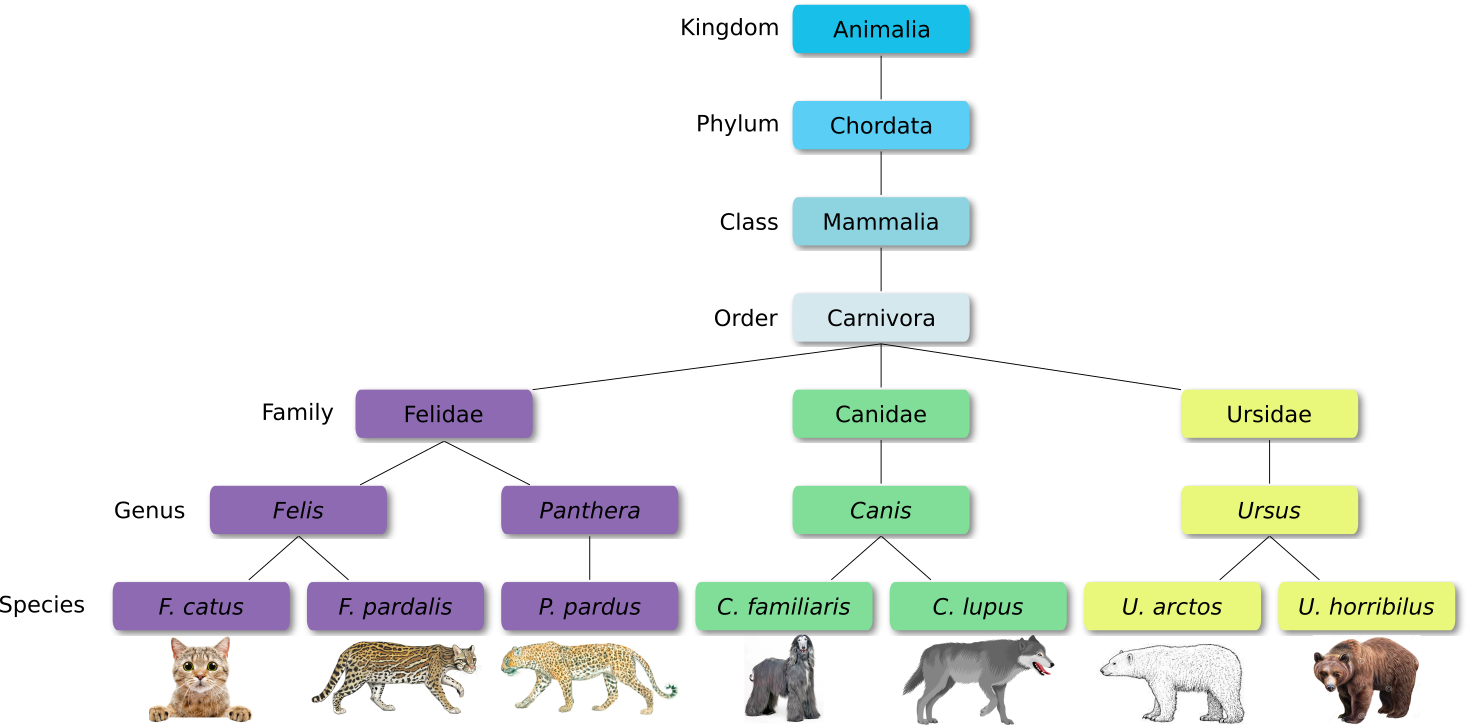
Taxonomy is the method used to naming, defining (circumscribing) and classifying groups of biological organisms based on shared characteristics such as morphological characteristics, phylogenetic characteristics, DNA data, etc. It is founded on the concept that the similarities descend from a common evolutionary ancestor.
Defined groups of organisms are known as taxa. Taxa are given a taxonomic rank and are aggregated into super groups of higher rank to create a taxonomic hierarchy. The taxonomic hierarchy includes eight levels: Domain, Kingdom, Phylum, Class, Order, Family, Genus and Species.
The classification system begins with 3 domains that encompass all living and extinct forms of life
- The Bacteria and Archae are mostly microscopic, but quite widespread.
- Domain Eukarya contains more complex organisms
When new species are found, they are assigned into taxa in the taxonomic hierarchy. For example for the cat:
Level Classification Domain Eukaryota Kingdom Animalia Phylum Chordata Class Mammalia Order Carnivora Family Felidae Genus Felis Species F. catus From this classification, one can generate a tree of life, also known as a phylogenetic tree. It is a rooted tree that describes the relationship of all life on earth. At the root sits the “last universal common ancestor” and the three main branches (in taxonomy also called domains) are bacteria, archaea and eukaryotes. Most important for this is the idea that all life on earth is derived from a common ancestor and therefore when comparing two species, you will -sooner or later- find a common ancestor for all of them.
Let’s explore taxonomy in the Tree of Life, using Lifemap
Question
- Which microorganisms do we expect to identify in our data?
- What is the taxonomy of the main expected microorganism?
The sequences are supposed to be yeasts extracted from a bottle of beer. The majority of beers contain a yeast genus called Saccharomyces and 2 species in that genus: Saccharomyces cerevisiae (ale yeast) and Saccharomyces pastorianus (lager yeast). The used beer is an ale beer, so we expect to find Saccharomyces cerevisiae. But other yeasts can also have been used and then found. We could also have some DNA left from other beer components, but also contaminations by other microorganisms and even human DNA from people who manipulated the beer or did the extraction.
The main expected microorganism is Saccharomyces cerevisiae with its taxonomy:
Level Classification Domain Eukaryota Kingdom Fungi Phylum Ascomycota Class Saccharomycetes Order Saccharomycetales Family Saccharomycetaceae Genus Saccharomyces Species S. cerevisiae
Taxonomic assignment or classification is the process of assigning an Operational Taxonomic Unit (OTUs, that is, groups of related individuals / taxon) to sequences. To assign an OTU to a sequence it is compared against a database, but this comparison can be done in different ways, with different bioinformatics tools. Here we will use Kraken2 (Wood et al. 2019).
In the \(k\)-mer approach for taxonomy classification, we use a database containing DNA sequences of genomes whose taxonomy we already know. On a computer, the genome sequences are broken into short pieces of length \(k\) (called \(k\)-mers), usually 30bp.
Kraken examines the \(k\)-mers within the query sequence, searches for them in the database, looks for where these are placed within the taxonomy tree inside the database, makes the classification with the most probable position, then maps \(k\)-mers to the lowest common ancestor (LCA) of all genomes known to contain the given \(k\)-mer.
Kraken2 uses a compact hash table, a probabilistic data structure that allows for faster queries and lower memory requirements. It applies a spaced seed mask of s spaces to the minimizer and calculates a compact hash code, which is then used as a search query in its compact hash table; the lowest common ancestor (LCA) taxon associated with the compact hash code is then assigned to the k-mer.
You can find more information about the Kraken2 algorithm in the paper Improved metagenomic analysis with Kraken 2.
 of the genomes that contain that k-mer in the database. The taxa associated with the sequence's k-mers, as well as the taxa's ancestors, form a pruned subtree of the general taxonomy tree, which is used for classification. In the classification tree, each node has a weight equal to the number of k-mers in the sequence associated with the node's taxon. Each root-to-leaf (RTL) path in the classification tree is scored by adding all weights in the path, and the maximal RTL path in the classification tree is the classification path (nodes highlighted in yellow). The leaf of this classification path (the orange, leftmost leaf in the classification tree) is the classification used for the query sequence. Source: <span class=\"citation\"><a href=\"#Wood2014\">Wood and Salzberg 2014</a></span>")
Hands On: Kraken2
- Kraken2 ( Galaxy version 2.1.1+galaxy1) with the following parameters:
- “Single or paired reads”:
Single
- param-file “Input sequences”: Output of fastp
- “Print scientific names instead of just taxids”:
Yes- In “Create Report”:
- “Print a report with aggregrate counts/clade to file”:
Yes“Select a Kraken2 database”:
Prebuilt Refseq indexes: PlusPFThe database here contains reference sequences and taxonomies. We need to be sure it contains yeasts, i.e. fungi.
- Inspect the report file
The Kraken report is a tabular files with one line per taxon and 6 columns or fields:
- Percentage of fragments covered by the clade rooted at this taxon
- Number of fragments covered by the clade rooted at this taxon
- Number of fragments assigned directly to this taxon
- A rank code, indicating
- (U)nclassified
- (R)oot
- (D)omain
- (K)ingdom
- (P)hylum
- (C)lass
- (O)rder
- (F)amily
- (G)enus, or
- (S)pecies
Taxa that are not at any of these 10 ranks have a rank code that is formed by using the rank code of the closest ancestor rank with a number indicating the distance from that rank. E.g.,
G2is a rank code indicating a taxon is between genus and species and the grandparent taxon is at the genus rank. - NCBI taxonomic ID number
- Indented scientific name
Column 1	Column 2	Column 3	Column 4	Column 5	Column 6
38.00 	513 	513 	U 	0 	unclassified
62.00 	837 	1 	R 	1 	root
61.93 	836 	27 	R1 	131567 	cellular organisms
56.00 	756 	3 	D 	2759 	Eukaryota
55.33 	747 	3 	D1 	33154 	Opisthokonta
29.78 	402 	0 	K 	33208 	Metazoa
29.78 	402 	0 	K1 	6072 	Eumetazoa
29.78 	402 	0 	K2 	33213 	Bilateria
29.78 	402 	0 	K3 	33511 	Deuterostomia
29.78 	402 	0 	P 	7711 	Chordata
29.78 	402 	0 	P1 	89593 	Craniata
29.78 	402 	0 	P2 	7742 	Vertebrata
29.78 	402 	0 	P3 	7776 	Gnathostomata
29.78 	402 	0 	P4 	117570 	Teleostomi
29.78 	402 	0 	P5 	117571 	Euteleostomi
29.78 	402 	0 	P6 	8287 	Sarcopterygii
29.78 	402 	0 	P7 	1338369 	Dipnotetrapodomorpha
29.78 	402 	0 	P8 	32523 	Tetrapoda
29.78 	402 	0 	P9 	32524 	Amniota
29.78 	402 	0 	C 	40674 	Mammalia
Question
- How many taxons have been identified?
- How much reads have been classified?
- Which domains were found and with how many reads?
- How much reads have been assigned by fungi Kingdom?
The file contains 300 lines (information visible when expanding the report dataset in the history panel). So 300-2 = 298 taxons have been identified.
On the 1350 sequences in the input, 837 (62%) were classified (or identified as a taxon) and 513 unclassified (38%). Information visible when expanding the report dataset in the history panel, and scrolling in the small box starting with “Loading database information” below the format information, but also on the top of the report.
The domains are identified by a
Din colum 4.To get the domains (or other taxonomic level), we can use Filter with the following parameters:
- param-file “Filter”: report outpout of Kraken2
- “With following condition”:
c4=='D'The 3 domains were found:
- Eukaryota with 756 (56%) reads assigned to it
- Bacteria with 51 (3.78%) reads
- Archaea with 2 (0.15%) reads
342 (25.33%) reads are assigned to fungi.
Other taxons than yeast have been identified. They could be contamination or misidentification of reads. Indeed, many taxons have less than 5 reads assigned. We will filter these reads out to get a better view of the possible contaminations.
Hands On: Filter taxons with low assignements
- Filter with the following parameters:
- param-file “Filter”: report outpout of Kraken2
“With following condition”:
c2>5We want to keep only taxons with more than 5 reads assigned, i.e. the value in the 2nd column, is higher than 5.
- Inspect the output
Question
- How many taxons have been removed? How many were kept?
- What are the possible contaminations?
59 lines are now in the file so \(300 - 59 = 241\) taxons have been removed because low assignment rates.
Most of the reads (402) were assigned to humans (Homo sapiens). This is likely a contamination either during the beer production or more likely during DNA extraction.
Bacteria were also found: Firmicutes, Proteobacteria and Bacteroidetes. But the identified taxons are not really precise (not below order level). So difficult to identify the possible source of contamination.
Visualize the community
Once we have assigned the corresponding taxa to the sequences, the next step is to properly visualize the data: visualize the diversity of taxons at different levels.
To do that, we will use the tool Krona (Ondov et al. 2011). But before that, we need to adjust the output from Kraken2 to the requirements of Krona. Indeed, Krona expects as input a table with the first column containing a count and the remaining columns describing the hierarchy. Currently, we have a report tabular file with the first column containing the taxonomy and the second column the number of reads. We will now use another tool, which also provides taxonomic classification, but it produces the exact formatting Krona needs.
Hands On: Prepare dataset for Krona
- Krakentools: Convert kraken report file ( Galaxy version 1.2+galaxy0) with the following parameters:
- param-collection “Kraken report file”: Report output of Kraken
Inspect the output file
QuestionColumn 1 Column 2 Column 3 Column 4 Column 5 Column 6 Column 7 Column 8 513 Unclassified 7 k__Eukaryota 0 k__Eukaryota p__Chordata 0 k__Eukaryota p__Chordata c__Mammalia 0 k__Eukaryota p__Chordata c__Mammalia o__Primates 0 k__Eukaryota p__Chordata c__Mammalia o__Primates f__Hominidae 0 k__Eukaryota p__Chordata c__Mammalia o__Primates f__Hominidae g__Homo 402 k__Eukaryota p__Chordata c__Mammalia o__Primates f__Hominidae g__Homo s__Homo_sapiens
- What are the columns in the file?
- 8 columns: one with the number of reads and one for each of the 7 levels of taxonomy.
We can now run Krona. This tool creates an interactive report that allows hierarchical data (like taxonomy) to be explored with zooming, as multi-layered pie charts. With this tool, we can easily visualize the composition of a microbiome community.
Hands On: Krona pie chart
- Krona pie chart ( Galaxy version 2.7.1+galaxy0) with the following parameters:
- “What is the type of your input data”:
Tabular
- param-file “Input file”: output of Krakentools tool
- Inspect the generated file
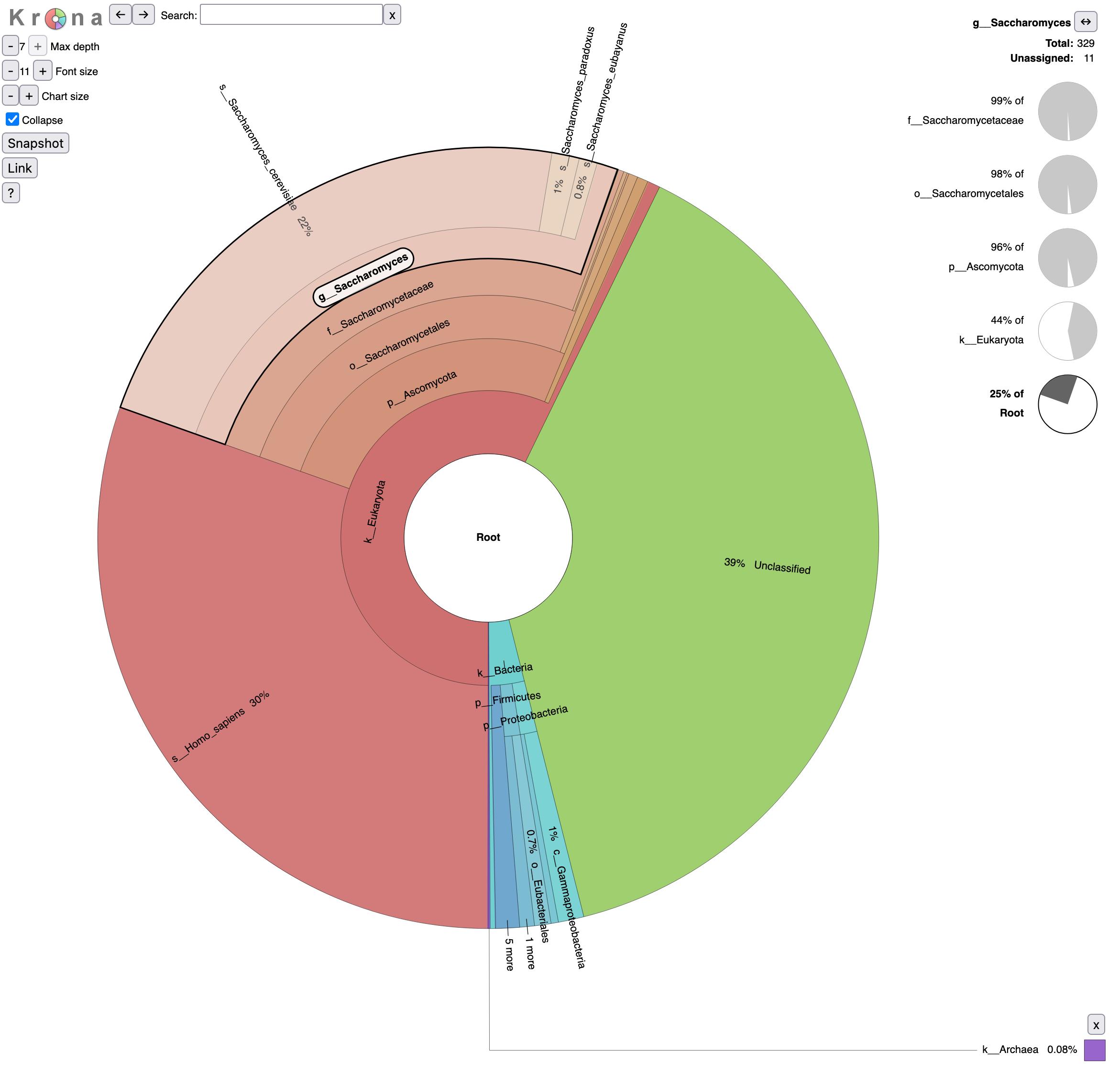
Let’s take a look at the result.
Question
- What is the percentage of reads assigned to Homo sapiens?
- To Archaea?
- 30% of reads are assigned to Homo sapiens
- 0.08% of Archaea
Investigate the beer microbiome
Let’s come back to our original question: characterization of the beer microbiome, specially looking at the yeasts.
Yeasts do not form a single taxonomic group (Kurtzman 1994). They are parts of the fungi kingdom but belong two separate phyla: the Ascomycota and the Basidiomycota. But the “true yeasts” are classified in the order Saccharomycetales.
Question
- Click on
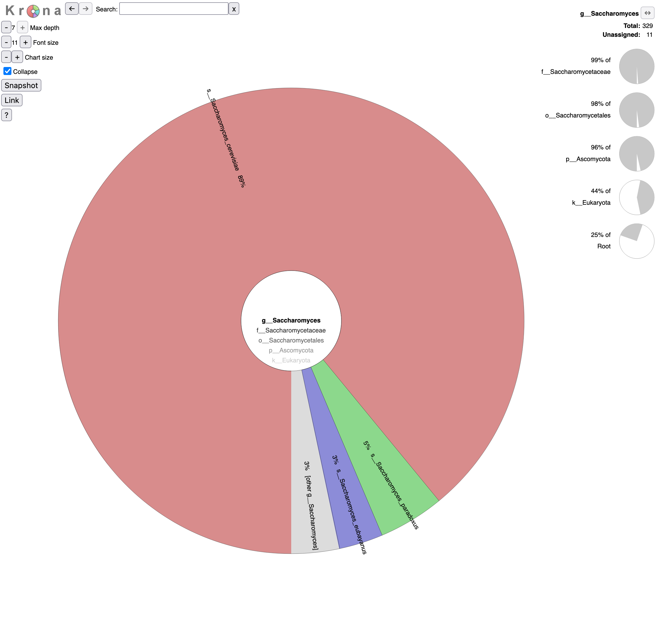
o__Saccharomycetalesin the graph (Krona pie chart). Which yeast species have been identified? Are they the expected in beer?- Click on Saccharomyces in the graph. What are the percentages of identified reads assigned to Saccharomyces for different levels?
- Click a second time on Saccharomyces in the graph. What is the repartition between the different Saccharomyces species?
- 6 species from the Saccharomycetales order have been identified:
- Saccharomycetaceae family
- Saccharomyces genus
- Saccharomyces cerevisiae species, the most abundant identified yeast species with 293 reads and the one expected given the type of beers
Saccharomyces paradoxus species, a wild yeast and the closest known species to Saccharomyces cerevisiae
These reads might have been misidentified to Saccharomyces paradoxus instead of Saccharomyces cerevisiae because of some errors in the sequences, as Saccharomyces cerevisiae and Saccharomyces paradoxus are close species and should share then a lot of similarity in their sequences.
Saccharomyces eubayanus species, most likely the parent of the lager brewing yeast, Saccharomyces pastorianus (Sampaio 2018)
Similar to Saccharomyces paradoxus, these reads might have been misassigned.
- Kluyveromyces genus - Kluyveromyces marxianus species: only 1 read
- Trichomonascaceae family - Sugiyamaella genus - Sugiyamaella lignohabitans species: only 1 read
- Debaryomycetaceae family - Candida genus - Candida dubliniensis species: only 1 read
Everything except Saccharomyces cerevisiae are probably misindentified reads.
- Reads are assigned to Saccharomyces
- 25% out of total reads (root)
- 44% out of identified reads for Eukaryota domain
- 96% out of identified reads for Ascomycota phylum
- 98% out of identified reads for Saccharomycetales order
- 99% out of identified reads for Saccharomycetaceae family
92% of Saccharomyces reads are assigned to Saccharomyces cerevisiae, 5% to Saccharomyces paradoxus and 3% to Saccharomyces eubayanus,.
Microbiome of several beers, including Chimay beers, have been previously investigated by targeting specifically the fungi, in which we can find yeasts (Sobel et al. 2017):
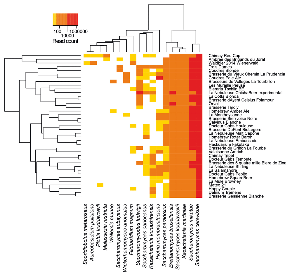 Open image in new tab
The species identified for Chimay beers are (from the most abundant to the least one):
- Saccharomyces cerevisiae
- Saccharomyces mikatea: a species generally used in winemaking (Bellon et al. 2013)
- Kazachstania martiniae: Kazachstania is a genus from the family Saccharomycetaceaethe.
- Saccharomyces kudriavzevii
-
Brettanomyces bruxellensis
Brettanomyces is a non-spore forming genus of yeast in the family Saccharomycetaceae, and is important to both the brewing and wine industries due to the sensory compounds it produces.
Brettanomyces bruxellensis is typically used for the production of the Belgian beers.
- Saccharomyces paradoxus: a wild yeast species closely related to Saccharomyces cerevisiae
- Kazachstania kunashirensis
- Saccharomyces cariocanus: a wild yeast species closely related to Saccharomyces cerevisiae
- Filobasidium magnum
- Malasseria restricta
- Pichia kudriavzevii
- Aureobasidium pullulans
- Sporidiobolus metaroseus
In a structured way:
| Phylum | Class | Order | Family | Genus | Species |
|---|---|---|---|---|---|
| Ascomycota | Saccharomycetes | Saccharomycetales | Saccharomycetaceae | Saccharomyces | Saccharomyces cerevisiae |
| Ascomycota | Saccharomycetes | Saccharomycetales | Saccharomycetaceae | Saccharomyces | Saccharomyces mikatea |
| Ascomycota | Saccharomycetes | Saccharomycetales | Saccharomycetaceae | Saccharomyces | Saccharomyces kudriavzevii |
| Ascomycota | Saccharomycetes | Saccharomycetales | Saccharomycetaceae | Saccharomyces | Saccharomyces paradoxus |
| Ascomycota | Saccharomycetes | Saccharomycetales | Saccharomycetaceae | Saccharomyces | Saccharomyces cariocanus |
| Ascomycota | Saccharomycetes | Saccharomycetales | Saccharomycetaceae | Kazachstania | Kazachstania martiniae |
| Ascomycota | Saccharomycetes | Saccharomycetales | Saccharomycetaceae | Kazachstania | Kazachstania kunashirensis |
| Ascomycota | Saccharomycetes | Saccharomycetales | Saccharomycetaceae | Brettanomyces | Brettanomyces bruxellensis |
| Ascomycota | Saccharomycetes | Saccharomycetales | Saccharomycetaceae | Pichia kudriavzevii | |
| Ascomycota | Dothideomycetes | Dothideales | Dothioraceae | Aureobasidium | Aureobasidium pullulans |
| Basidiomycota | Tremellomycetes | Filobasidiales | Filobasidiaceae | Filobasidium | Filobasidium magnum |
| Basidiomycota | Malasseziomycetes | Malasseziales | Malasseziaceae | Malassezia | Malasseria restricta |
| Basidiomycota | Sporidiobolales | Sporidiobolales | Sporidiobolaceae | Sporidiobolus | Sporidiobolus metaroseus |
QuestionBy looking at the output of Krakentools, which fungi species identified for the Chimay beers in Sobel et al. 2017 are also identified in our data? And vice versa?
Phylum Class Order Family Genus Species Sobel et al. 2017 Our data Ascomycota Saccharomycetes Saccharomycetales Saccharomycetaceae Saccharomyces Saccharomyces cerevisiae X X Ascomycota Saccharomycetes Saccharomycetales Saccharomycetaceae Saccharomyces Saccharomyces mikatea X Ascomycota Saccharomycetes Saccharomycetales Saccharomycetaceae Saccharomyces Saccharomyces kudriavzevii X Ascomycota Saccharomycetes Saccharomycetales Saccharomycetaceae Saccharomyces Saccharomyces paradoxus X X Ascomycota Saccharomycetes Saccharomycetales Saccharomycetaceae Saccharomyces Saccharomyces cariocanus X Ascomycota Saccharomycetes Saccharomycetales Saccharomycetaceae Saccharomyces Saccharomyces eubayanus X Ascomycota Saccharomycetes Saccharomycetales Saccharomycetaceae Kazachstania Kazachstania martiniae X Ascomycota Saccharomycetes Saccharomycetales Saccharomycetaceae Kazachstania Kazachstania kunashirensis X Ascomycota Saccharomycetes Saccharomycetales Saccharomycetaceae Kluyveromyces Kluyveromyces marxianus X Ascomycota Saccharomycetes Saccharomycetales Saccharomycetaceae Brettanomyces Brettanomyces bruxellensis X Ascomycota Saccharomycetes Saccharomycetales Saccharomycetaceae Pichia kudriavzevii X Ascomycota Saccharomycetes Saccharomycetales Debaryomycetaceae Candida Candida dubliniensis X Ascomycota Dothideomycetes Dothideales Dothioraceae Aureobasidium Aureobasidium pullulans X Ascomycota Sordariomycetes Sordariales Sordariaceae Neurospora Neurospora crassa X Basidiomycota Tremellomycetes Filobasidiales Filobasidiaceae Filobasidium Filobasidium magnum X Basidiomycota Malasseziomycetes Malasseziales Malasseziaceae Malassezia Malasseria restricta X Basidiomycota Sporidiobolales Sporidiobolales Sporidiobolaceae Sporidiobolus Sporidiobolus metaroseus X
Some interesting yeast have been found in Sobel et al. 2017 and not in our data (e.g. Brettanomyces bruxellensis), and vice versa.
(Optional) Sharing your history
One of the most important features of Galaxy comes at the end of an analysis: sharing your histories with others so they can review them.
Sharing your history allows others to import and access the datasets, parameters, and steps of your history.
Access the history sharing menu via the History Options dropdown (galaxy-history-options), and clicking “history-share Share or Publish”
- Share via link
- Open the History Options galaxy-history-options menu at the top of your history panel and select “history-share Share or Publish”
- galaxy-toggle Make History accessible
- A Share Link will appear that you give to others
- Anybody who has this link can view and copy your history
- Publish your history
- galaxy-toggle Make History publicly available in Published Histories
- Anybody on this Galaxy server will see your history listed under the Published Histories tab opened via the galaxy-histories-activity Histories activity
- Share only with another user.
- Enter an email address for the user you want to share with in the Please specify user email input below Share History with Individual Users
- Your history will be shared only with this user.
- Finding histories others have shared with me
- Click on the galaxy-histories-activity Histories activity in the activity bar on the left
- Click the Shared with me tab
- Here you will see all the histories others have shared with you directly
Note: If you want to make changes to your history without affecting the shared version, make a copy by going to History Options galaxy-history-options icon in your history and clicking Copy this History
Conclusion
You've Finished the Tutorial
Key points
Data obtained by sequencing needs to be checked for quality and cleaned before further processing
Yeast species but also contamination can be identified and visualized directly from the sequences using several bioinformatics tools
With its graphical interface, Galaxy makes it easy to use the needed bioinformatics tools
Beer microbiome is not just made of yeast and can be quite complex
Frequently Asked Questions
Have questions about this tutorial? Have a look at the available FAQ pages and support channelsUseful literature
Further information, including links to documentation and original publications, regarding the tools, analysis techniques and the interpretation of results described in this tutorial can be found here.
References
- Kurtzman, C. P., 1994 Molecular taxonomy of the yeasts. Yeast 10: 1727–1740. 10.1002/yea.320101306
- Ondov, B. D., N. H. Bergman, and A. M. Phillippy, 2011 Interactive metagenomic visualization in a Web browser. BMC Bioinformatics 12: 10.1186/1471-2105-12-385
- Bellon, J. R., F. Schmid, D. L. Capone, B. L. Dunn, and P. J. Chambers, 2013 Introducing a new breed of wine yeast: interspecific hybridisation between a commercial Saccharomyces cerevisiae wine yeast and Saccharomyces mikatae. PLoS one 8: e62053. 10.1371/journal.pone.0062053
- Wood, D. E., and S. L. Salzberg, 2014 Kraken: ultrafast metagenomic sequence classification using exact alignments. Genome Biology 15: R46. 10.1186/gb-2014-15-3-r46
- Sobel, J., L. Henry, N. Rotman, and G. Rando, 2017 BeerDeCoded: the open beer metagenome project. F1000Research 6: 1676. 10.12688/f1000research.12564.2
- Wick, R., 2017 Porechop. GitHub. https://github.com/rrwick/Porechop
- Chen, S., Y. Zhou, Y. Chen, and J. Gu, 2018 fastp: an ultra-fast all-in-one FASTQ preprocessor. 10.1101/274100
- Sampaio, J. P., 2018 Microbe profile: Saccharomyces eubayanus, the missing link to lager beer yeasts. Microbiology 164: 1069. 10.1099/mic.0.000677
- Wood, D. E., J. Lu, and B. Langmead, 2019 Improved metagenomic analysis with Kraken 2. Genome biology 20: 1–13. 10.1186/s13059-019-1891-0
- Delahaye, C., and J. Nicolas, 2021 Sequencing DNA with nanopores: Troubles and biases. PLoS One 16: e0257521. 10.1371/journal.pone.0257521
Feedback
Did you use this material as an instructor? Feel free to give us feedback on how it went.
Did you use this material as a learner or student? Click the form below to leave feedback.

Citing this Tutorial
- Polina Polunina, Siyu Chen, Bérénice Batut, Teresa Müller, Identification of the micro-organisms in a beer using Nanopore sequencing (Galaxy Training Materials). https://training.galaxyproject.org/training-material/topics/microbiome/tutorials/beer-data-analysis/tutorial.html Online; accessed TODAY
- Hiltemann, Saskia, Rasche, Helena et al., 2023 Galaxy Training: A Powerful Framework for Teaching! PLOS Computational Biology 10.1371/journal.pcbi.1010752
- Batut et al., 2018 Community-Driven Data Analysis Training for Biology Cell Systems 10.1016/j.cels.2018.05.012
@misc{microbiome-beer-data-analysis,
author = "Polina Polunina and Siyu Chen and Bérénice Batut and Teresa Müller",
	title = "Identification of the micro-organisms in a beer using Nanopore sequencing (Galaxy Training Materials)",
	year = "",
	month = "",
	day = "",
	url = "\url{https://training.galaxyproject.org/training-material/topics/microbiome/tutorials/beer-data-analysis/tutorial.html}",
	note = "[Online; accessed TODAY]"
}
@article{Hiltemann_2023,
	doi = {10.1371/journal.pcbi.1010752},
	url = {https://doi.org/10.1371%2Fjournal.pcbi.1010752},
	year = 2023,
	month = {jan},
	publisher = {Public Library of Science ({PLoS})},
	volume = {19},
	number = {1},
	pages = {e1010752},
	author = {Saskia Hiltemann and Helena Rasche and Simon Gladman and Hans-Rudolf Hotz and Delphine Larivi{\`{e}}re and Daniel Blankenberg and Pratik D. Jagtap and Thomas Wollmann and Anthony Bretaudeau and Nadia Gou{\'{e}} and Timothy J. Griffin and Coline Royaux and Yvan Le Bras and Subina Mehta and Anna Syme and Frederik Coppens and Bert Droesbeke and Nicola Soranzo and Wendi Bacon and Fotis Psomopoulos and Crist{\'{o}}bal Gallardo-Alba and John Davis and Melanie Christine Föll and Matthias Fahrner and Maria A. Doyle and Beatriz Serrano-Solano and Anne Claire Fouilloux and Peter van Heusden and Wolfgang Maier and Dave Clements and Florian Heyl and Björn Grüning and B{\'{e}}r{\'{e}}nice Batut and},
	editor = {Francis Ouellette},
	title = {Galaxy Training: A powerful framework for teaching!},
	journal = {PLoS Comput Biol}
}
Funding
These individuals or organisations provided funding support for the development of this resource
Congratulations on successfully completing this tutorial!You can use Ephemeris's
shed-tools installcommand to install the tools used in this tutorial.shed-tools install [-g GALAXY] [-a API_KEY] -t <(curl https://training.galaxyproject.org/training-material/api/topics/microbiome/tutorials/beer-data-analysis/tutorial.json | jq .admin_install_yaml -r)Alternatively you can copy and paste the following YAML
---
install_tool_dependencies: true
install_repository_dependencies: true
install_resolver_dependencies: true
tools:
- name: taxonomy_krona_chart
  owner: crs4
  revisions: e9005d1f3cfd
  tool_panel_section_label: Metagenomic Analysis
  tool_shed_url: https://toolshed.g2.bx.psu.edu/
- name: fastqc
  owner: devteam
  revisions: 3d0c7bdf12f5
  tool_panel_section_label: FASTA/FASTQ
  tool_shed_url: https://toolshed.g2.bx.psu.edu/
- name: fastp
  owner: iuc
  revisions: 65b93b623c77
  tool_panel_section_label: FASTA/FASTQ
  tool_shed_url: https://toolshed.g2.bx.psu.edu/
- name: kraken2
  owner: iuc
  revisions: 20e2f64aa1fe
  tool_panel_section_label: Metagenomic Analysis
  tool_shed_url: https://toolshed.g2.bx.psu.edu/
- name: krakentools_kreport2krona
  owner: iuc
  revisions: 88d274322340
  tool_panel_section_label: Metagenomic Analysis
  tool_shed_url: https://toolshed.g2.bx.psu.edu/
- name: porechop
  owner: iuc
  revisions: 543cbeef3949
  tool_panel_section_label: Nanopore
  tool_shed_url: https://toolshed.g2.bx.psu.edu/