Introduction to proteomics, protein identification, quantification and statistical modelling
Contributors
Proteomics
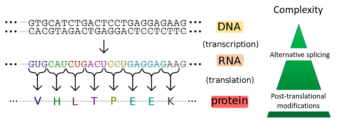
“A Proteome is the entire complement of proteins that is or can be expressed by a cell, tissue, or organism at a given time.” - Marc Wilkins 1996
.footnote[Image credit: Madprime]
Speaker Notes
Proteins are macromolecules that have many important functions in a cell. Protein coding genes are transcribed into mRNA, which is translated into amino acids. The amino acid chain forms secondary, tertiary and quartary structures to obtain a functional protein. One gene may generate different proteins due to alternative splicing and post-translational modifications. Therefore, the proteome level shows a higher molecular complexity. The proteome is defined as the entirety of proteins expressed by a genome or by a cell or tissue at a given time. The study of proteins is important as their identity and abundance is only partially predictable from DNA and mRNA information. This is due to alternative splicing, post-translational modifications, protein turnover and subcellular localization.
Mass Spectometry (MS)-based Proteomics
.force-right[
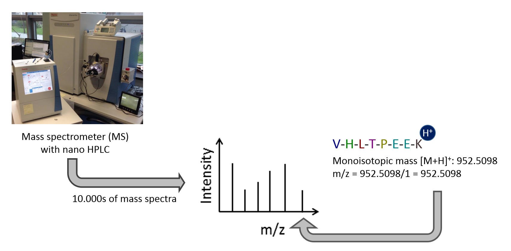
- Bottom-up approach: measurement of peptides after enzymatic digestion of proteins
- Measures the peptides mass-to-charge (m/z) ratio and stores m/z – intensity pairs in mass spectra
- High sensitivity and throughput
- Standard method for the analysis of complex samples ]
Speaker Notes
Mass spectrometry is the standard method for proteomic analyses of complex samples. In the classical bottom-up approach, proteins are enzymatically digested into peptides. Peptides can be analyzed with high sensitivity and throughput in a mass spectrometer. The peptide mass is measured as mass-to-charge ratio. Only charged peptides can be measured in the mass spectrometer. Tens of thousands of mass spectra are generated per sample. Each spectrum consists of many mass-to-charge and intensity pairs.
MS-based Proteomic Techniques
.image-90[ ] ] |
.image-90[ ] ] |
.image-90[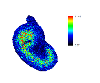 ] ] |
| Explorative Proteomics | Targeted Proteomics | Mass Spectometry |
| (DDA/DIA) | (SRM/PRM) | Imaging |
| All proteins of a cell/organ(ism) | Focus on subset of proteins | Focus on location of proteins |
Speaker Notes
Different mass spectrometry based proteomic techniques exist. The most common one is explorative or shotgun proteomics. It aims to identify as many proteins as possible from a sample. It comes in two flavours: data dependent acquisition (DDA) and data independent acquisition (DIA). A second technique is targeted proteomics. It measures only a predefined set of proteins with very accurate quantification. A third technique is mass spectrometry imaging. It measures the spatial distribution of peptides or proteins in thin tissue sections.
Proteomics tools in Galaxy
Speaker Notes
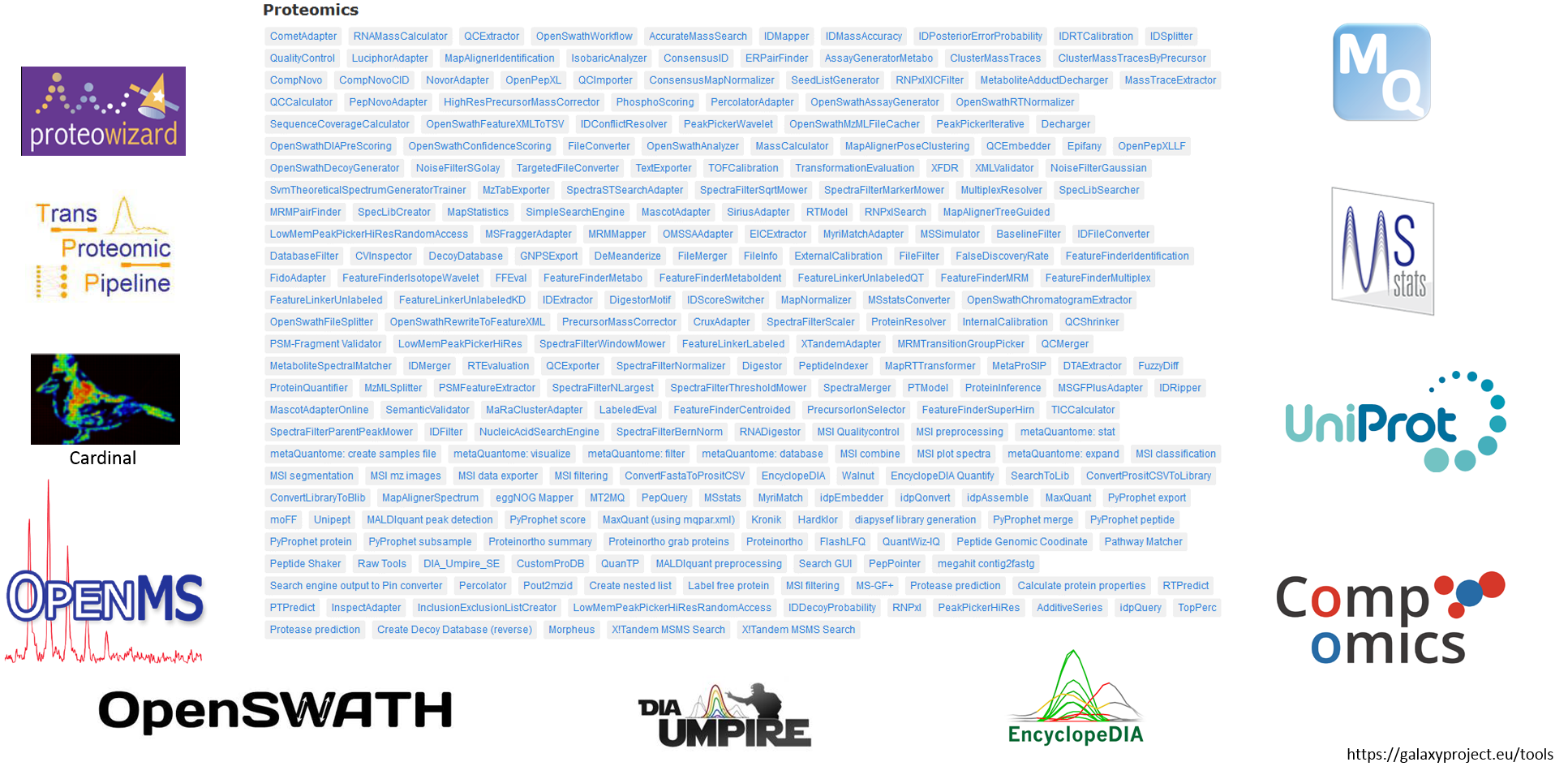
Plenty of software for DDA, D I A and mass spectrometry imaging are available in Galaxy. Here is an overview of all Proteomics tools installed on the European Galaxy Server. Other public Galaxy servers offer a similar or complementary proteomic tool kit. The Galaxy proteomics tools and training materials are constantly expanding and improving.
Explorative Proteomics
(DDA/DIA)
All proteins of a cell / organ / organism
Speaker Notes
This presentation will focus on explorative proteomics via the traditional DDA approach.
Explorative Proteomics Workflow
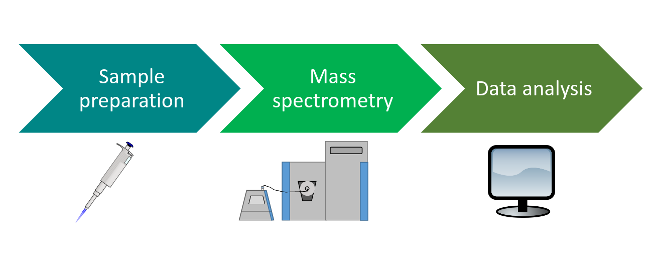
Speaker Notes
Proteomics experiments consist of three main steps. First, the sample is prepared for the analysis in the mass spectrometer. Then the sample is measured in the mass spectrometer. Last, the obtained data is analyzed.
class: top

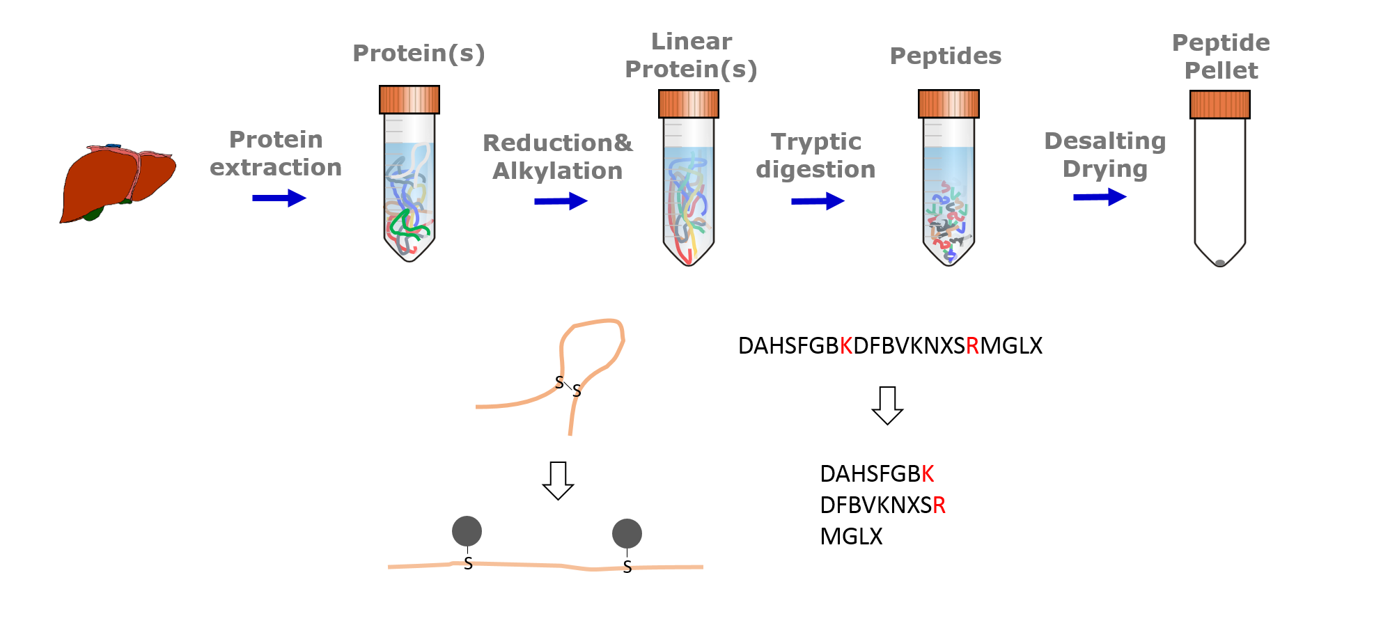
Speaker Notes
Typical sample preparation steps include protein extraction, reduction and alkylation, tryptic digestion and desalting. Before tryptic digestion, disulfide bridges are reduced and cysteins alkylated. This ensures that tryptic peptides are separated from each other and allows their mass based identification. Trypsin cleaves the amino acid sequences C-terminal of arginin and lysine. Desalting is a clean up step to protect the instrument from contamination and clogging.
class: top

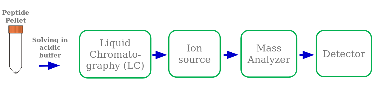
Speaker Notes
Sample measurement in a mass spectrometer consists of different steps. A high performance liquid chromatography (HPLC) system is attached in front of the mass spectrometer. It separates the injected peptide mixture according to their hydrophobicity. The peptides elute from the LC column into the mass spectrometer within several minutes to hours. This reduces sample complexity and gives the mass spectrometer more time for the measurement. The acidic LC buffer charges the peptides positively at their N-terminus and the basic lysin or arginin amino acids on the C-terminus. The LC column is directly connected with the ion source needle. There, high voltage and heat are applied to evaporate the ionized peptides into the gas phase. This process is called electrospray ionization. Inside the mass spectrometer the mass analyzer separates peptides based on their mass-to-charge ratio. The detector detects the peptide ions.
class: top
Liquid chromatography tandem mass spectrometry (LC-MS/MS)
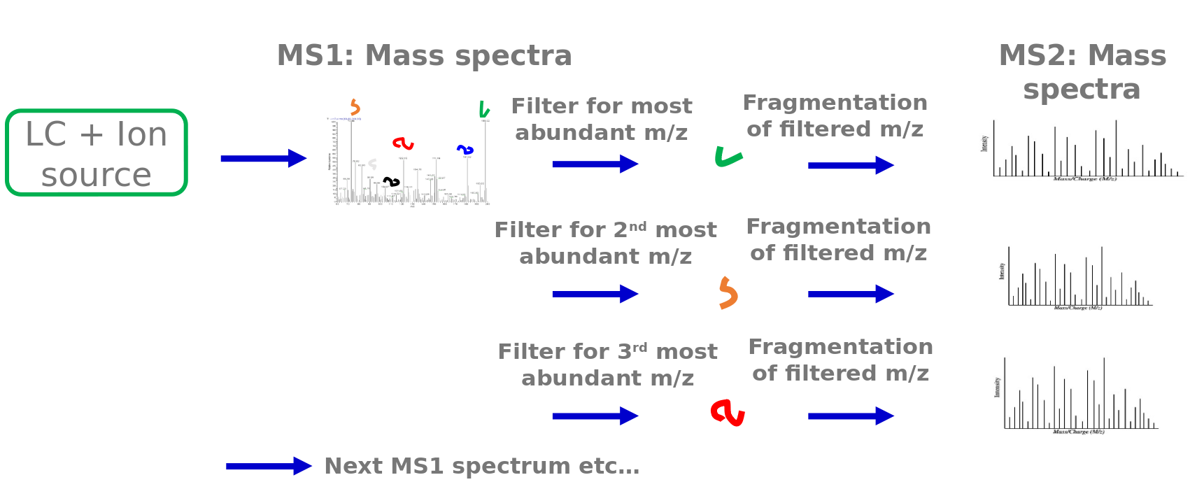
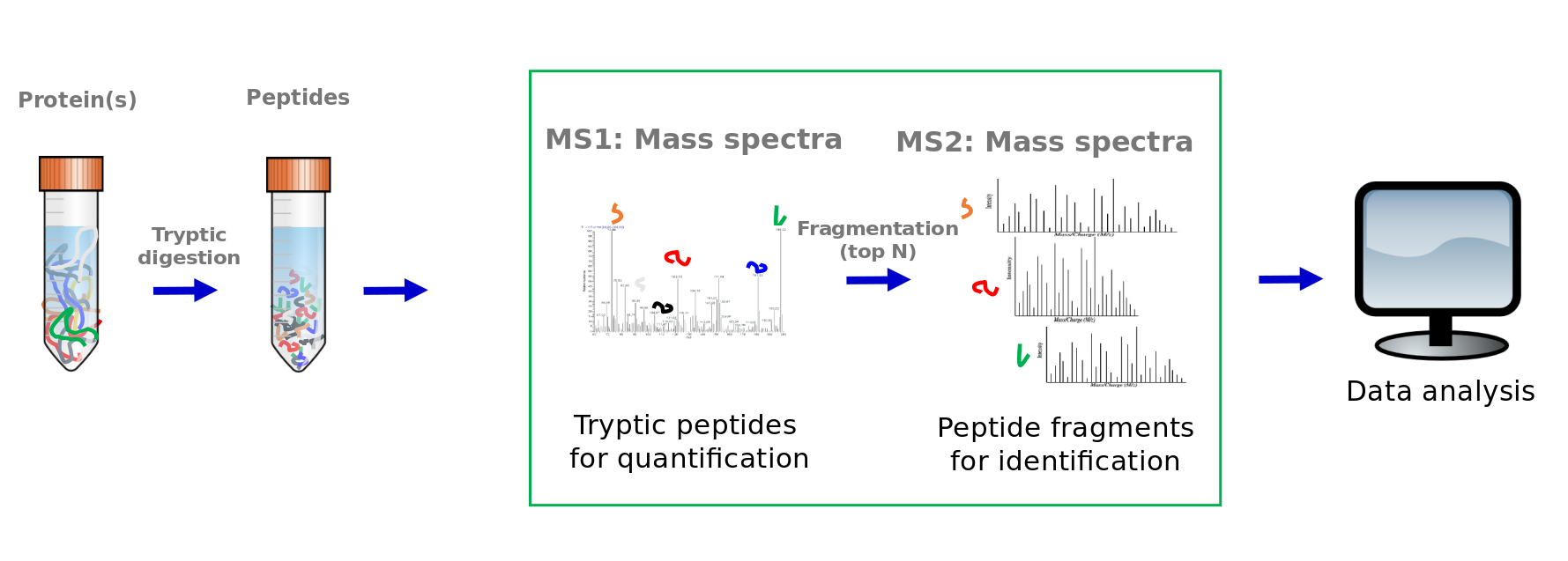
Speaker Notes
Typically explorative proteomics is performed via liquid chromatography tandem mass spectrometry (LC-MSMS). While the sample elutes from the LC column, thousands of mass spectra are acquired. First, a mass spectrum of all peptides at this time point is measured. These mass spectra are called MS1 spectra. From these spectra the N most abundant peptide peaks are determined. These topN peptides get fragmented. N is typically between 3 and 20. This example shows a Top3 method. The filter unit of the mass spectrometer (a quadrupole) allows only these peptides to pass. One after the other is selected in the filter unit and then fragmented by collision with neutral gas molecules. This fragmentation breaks the peptide bonds and generates peptide fragments. The peptide fragments are measured again via the mass analyzer and detector. These spectra are called MS2 spectra. After all topN peptides were fragmented and measured, another full MS1 mass spectra is acquired. MS1 and MS2 spectra are acquired in this way during the elution of the sample from the LC.
class: top

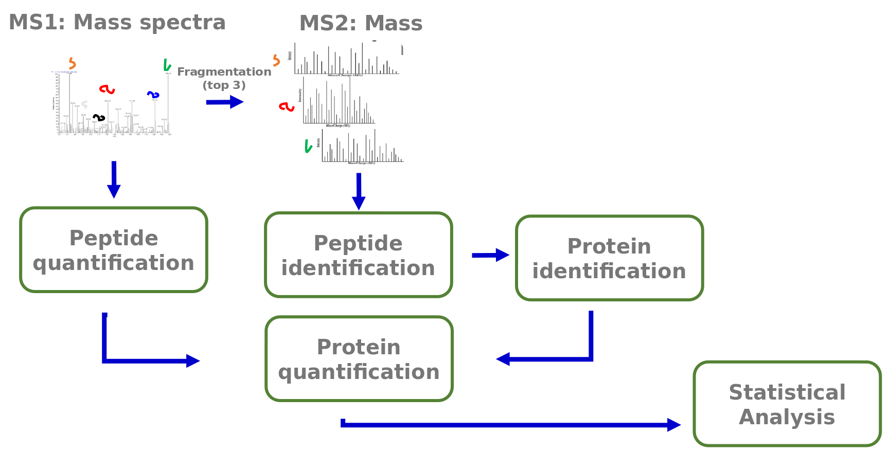
Speaker Notes
The analysis of the acquired mass spectra comprises several steps. First peptides are identified via their MS2 fragmentation spectra. From these peptide identities the corresponding proteins are assembled. The MS1 spectra are used for peptide quantification. Peptide quantities are summarized into protein quantities. The information about protein identity and quantity allows following statistical analyses.
Typical explorative tandem mass spectrometry workflow

Speaker Notes
This was the overview of a typical explorative tandem mass spectrometry workflow. Now we will dive into more details of the data analysis part.
Peptide identification with MS2 fragment spectra
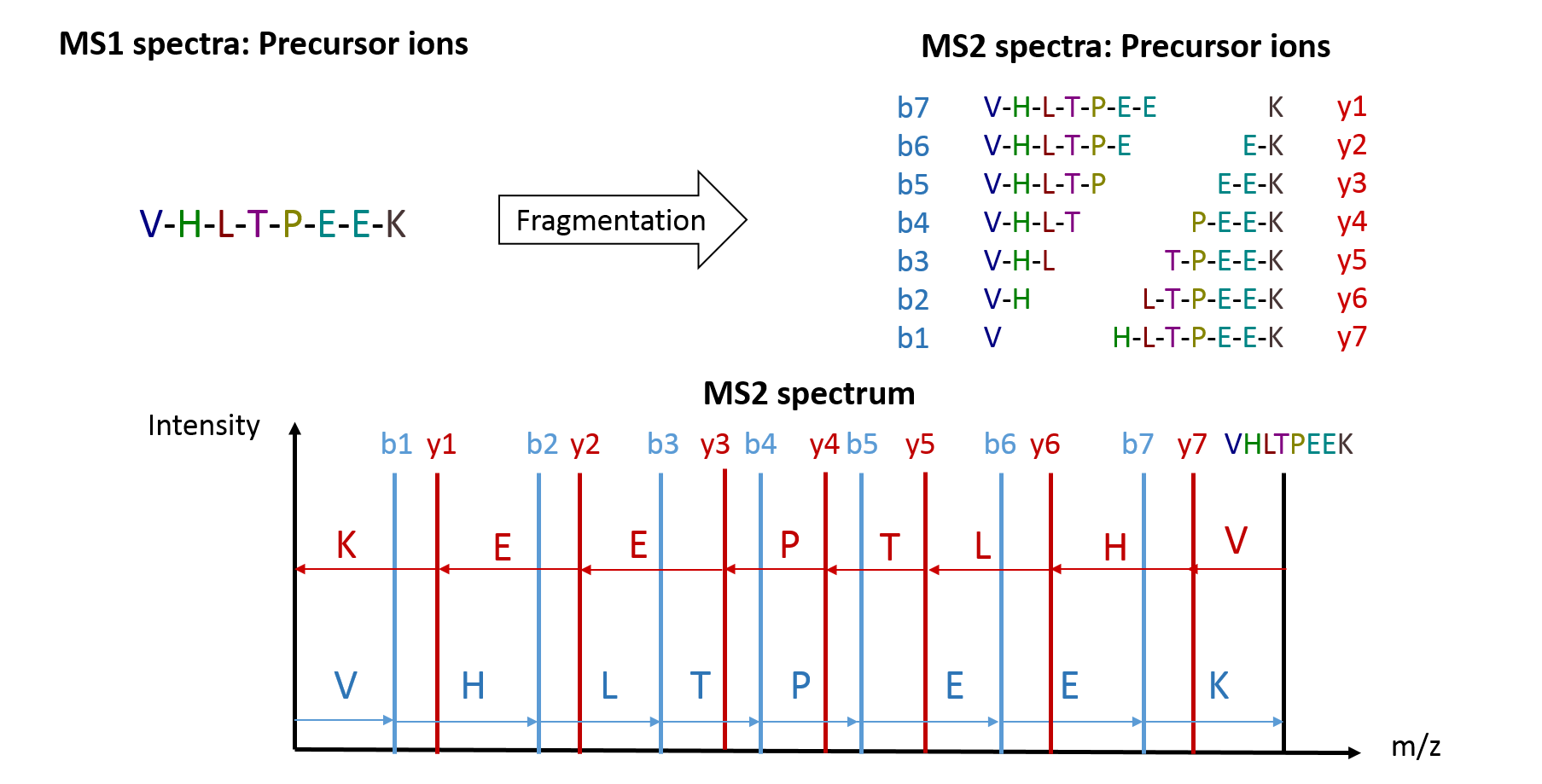
Speaker Notes
Many tryptic peptides of an organism have same or similar masses. Therefore, MS1 spectra don’t allow reliable peptide sequence identifications. MS2 spectra allow peptide identification via the generated peptide fragments. The N-terminal fragments are called b-ions and the C-terminal fragments y-ions. The differences between the fragment masses correspond to the mass of an amino acid. This allows manual interpretation of the spectra. However, this is a tricky procedure because in reality the MS2 spectra contain more noise and side product peaks than shown here. Also, in explorative proteomics tens of thousands of spectra are acquired and make manual interpretation unfeasible. The manual interpretation process is automatized with so called ‘de novo sequencing’ software. These algorithms have improved in the last years. No information about potential protein sequences in the sample are needed. The default software for peptide identification are so called ‘search engines’. They require information about all protein sequences of the analyzed organism as FASTA database. From this they generate in silico spectra which are then matched to the measured mass spectra.
Peptide spectrum matching
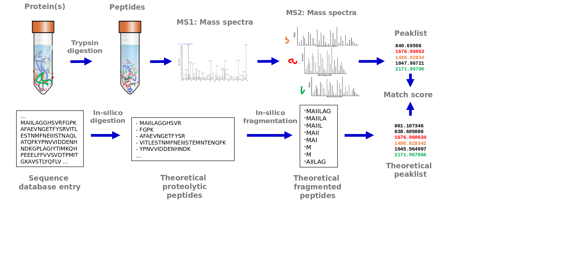
Speaker Notes
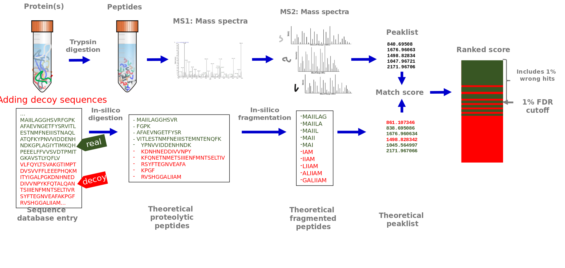
This process is often called ‘peptide spectrum matching’. It starts with a protein sequence database of all protein sequences of the analyzed organism. Analogous to the procedure in the sample, the protein sequences are in silico digested. This means that the sequences are cut after each lysine and arginin. These in silico tryptic peptide sequences are then in silico fragmented. All amino acid bonds may potentially break and generate peptide fragments. Therefore, all possible fragments are generated in silico. From each in silico peptide fragment, the mass is calculated. In case of amino acid modifications the mass of the modification is added accordingly. Fixed modifications are added to each occurrence of the amino acid on which they occur. Variable modifications may not occur on every amino acid and therefore two masses, with and without the modification, are calculated. These in silico generated mass values are matched to the mass values from each measured MS2 spectra. A matching score allows to find the best identifications for each MS2 spectrum.
Peptide spectrum matching
Speaker Notes
Potentially false matches may occur, therefore the false positive rate is controlled. This is done by adding decoy sequences to the protein sequence database. These sequences are generated by reversing or shuffling the real sequences and will not exist in the sample. In case such sequences are considered a good match to an MS2 spectra, this is a false match. One option to control the number of false positive matches is via a false discovery cutoff, that includes the best matching scores with only 1 % wrong decoy matches included.
FASTA File Format
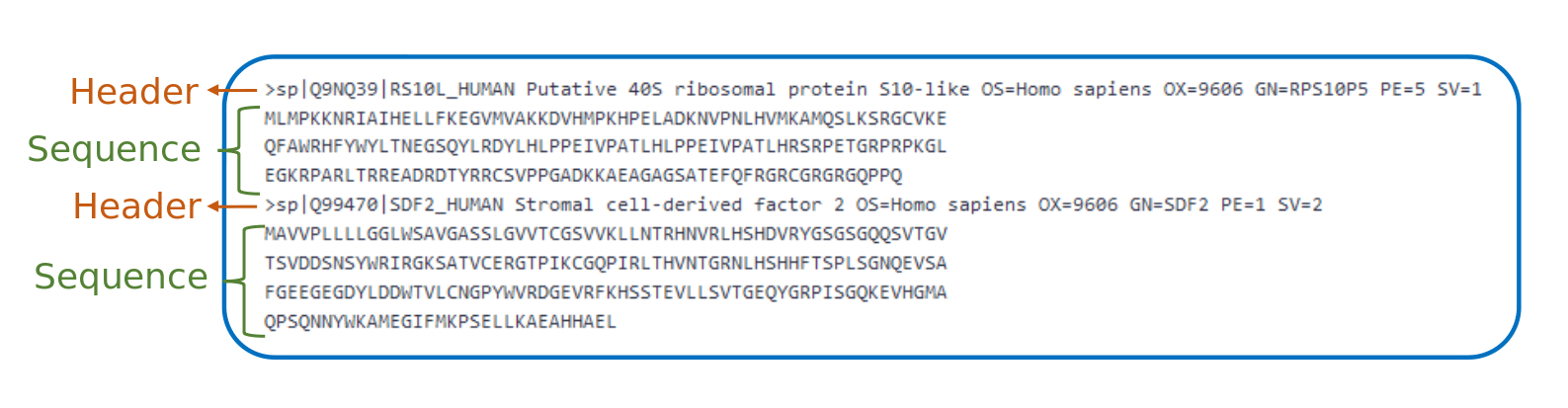
- Text based file to store DNA, RNA, protein sequences in a single letter code
- Each entry has
- One header line: starting with
>and containing a unique identifier - A (nucleotide/amino acid) sequence
- One header line: starting with
Speaker Notes
The protein sequence database is stored in a FASTA file. This is a text based file to store DNA, RNA or protein sequences in a single letter code. Each entry contains a header line and the sequence. The header line starts with a > and is follwed by a unique identifier.
FASTA Files for Proteomics
-
A proteome is the set of proteins thought to be expressed by an organism.
-
Only proteins that are present in the FASTA file can be identified
- The more proteins are present in the FASTA file the higher the changes for false identifications
- Choose the right FASTA file
- Source for proteome FASTA files:
- Uniprot, neXtProt, NCBI, own/public DNA or RNA sequencing data
.footnote[ Tutorial: Protein FASTA database handling ]
Speaker Notes
A proteome is the set of proteins thought to be expressed by an organism. Only proteins that are present in the FASTA file can be identified. But the more proteins are present in the FASTA file the higher the chances for false identifications and the longer the computation time. Sources for proteome FASTA files include uniprot, nextprot, NCBI or DNA and RNA sequencing data.
Protein Identification via Protein Inference
Speaker Notes
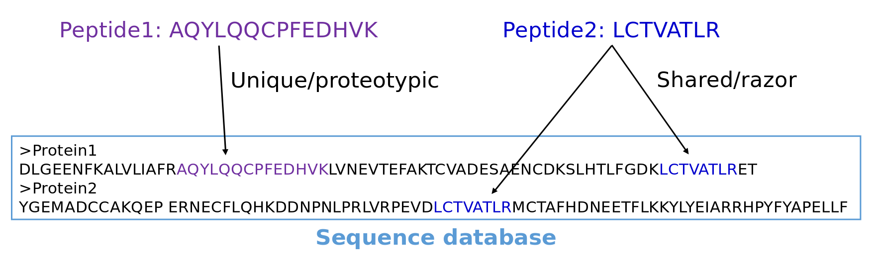
After having identified peptides, they need to be reconstructed into proteins. This step is called protein inference and is not trivial. Unique or proteotypic peptide sequences belong to one protein. But other peptide sequences may belong to several proteins. These peptides are called shared or razor peptides. Most protein inference algorithms assign them to the protein that has the most other peptides. In the depicted example peptide two would be matched to protein one which is for sure present in the sample because it has one unique peptide.
Quantification methods in proteomics
.footnote[ Tutorial: Label-free versus Labelled: How to Choose Your Quantitation Method]
Speaker Notes
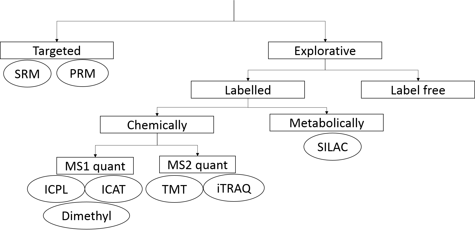
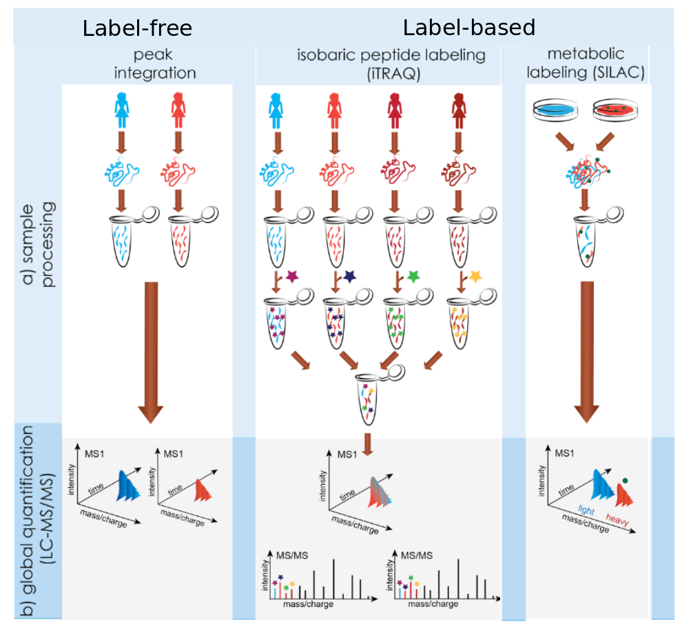
Different quantification approaches exist in mass spectrometry based proteomics. In explorative proteomic approaches relative quantification methods are applied. They compare the amount of proteins between different samples. Label-free and label based methods exist. Labels add specific mass tags to the peptides of different samples via metabolic or chemical ways.
Quantification Methods in Proteomics
.footnote[Image credit: Käll and Vitek 2011]
Speaker Notes
In label-free approaches every sample is measured separately. Afterwards, the protein amounts are compared between measurements. Chemical labeling techniques add a mass label to the digested peptide. Afterwards the samples are mixed and measured in one run. The different masses of the added labels allow distinguishing the origin of the proteins during data analysis. Depending on the labeling technique, up to 16 different labels exist. In metabolic labeling amino acids with heavy isotopes are added to the cell culture medium of one condition. During cell growth these amino acids get incorporated into proteins. Thus, proteins of the heavy condition can be distinguished by their normal counterparts via a fixed mass shift.
Label-free Peptide Quantification
Speaker Notes
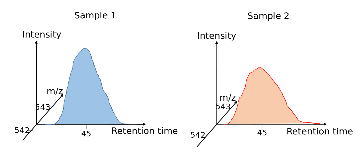
For label-free quantification all peak areas in the MS1 spectra are integrated.
Protein Quantification
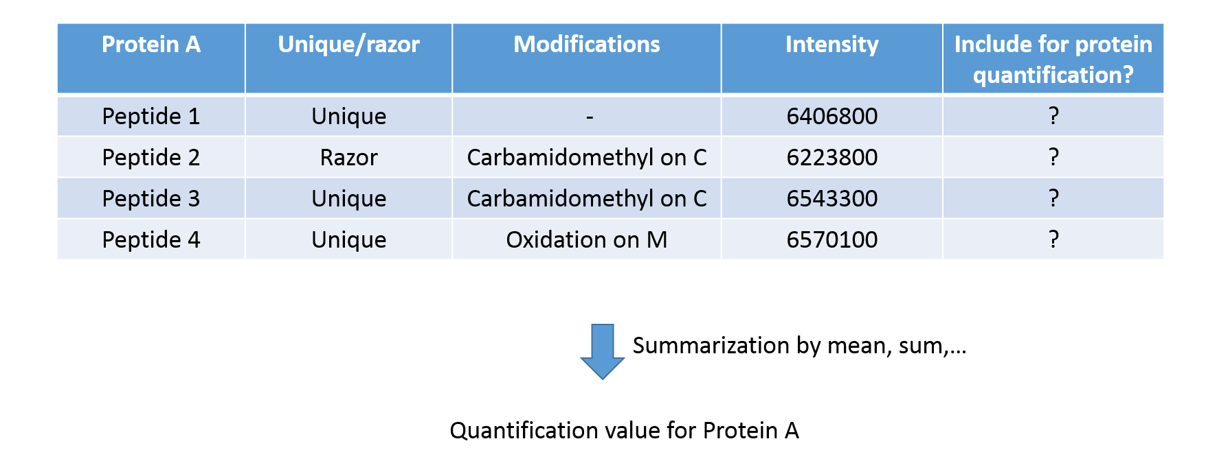
- Include only unique or also ambiguous razor peptides?
- Include peptides with modifications?
- How to summarize peptide abundances into protein abundances?
Speaker Notes
Peptide abundances are summarized into protein quantifications. This requires decisions about which peptides to include in the summarization. Only unique peptides? Only proteins with or without modifications? Last, the protein abundance may be computed by taking the median, mean, weighted mean or sum of all its peptides.
MaxQuant Software
.left-column50[
.image-100[
 ]
]
- Freeware, “Black Box”
- Popular non-commercial proteomics software ]
.right-column50[
- Raw data import
- Protein Identification:
- Andromeda Search Engine
- Protein Quantification:
- Label-free
- Label-based
- SILAC, Dimethyl, …
- Reporter ion MS2
- TMT, iTRAQ ]
.footnote[ Watch: MaxQuant videos on YouTube ]
Speaker Notes
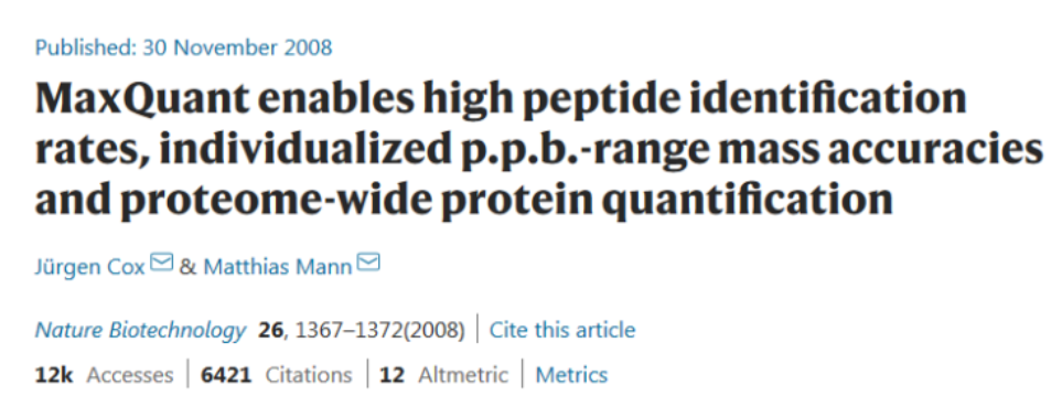
MaxQuant is the most popular non-commercial software for quantitative proteomics experiments. It performs protein identification via its Andromeda search engine. Protein quantification of label-free and many label-based methods is supported as well. MaxQuant accepts raw data in vendor specific formats.
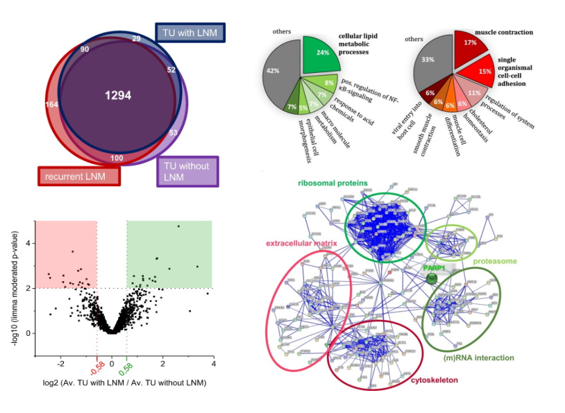
Follow up / Statistical Analysis
.pull-left[ Typical follow up procedures:
- Visualization
- E.g. venn-diagramm, volcano plot, heatmap, boxplots, histogram
-
Protein-Protein interaction network analysis
-
GO annotation and enrichment analysis
- Differentially abundant protein analysis
]
.pull-right[
.image-100[
 ]
]
]
]
.footnote[ Exemplary visualizations taken from Müller, 2018, Neoplasia ]
Speaker Notes
Typical follow up analyses include visualization, network and GO enrichment analysis. Finding differentially abundant proteins between different groups requires statistical analyses.
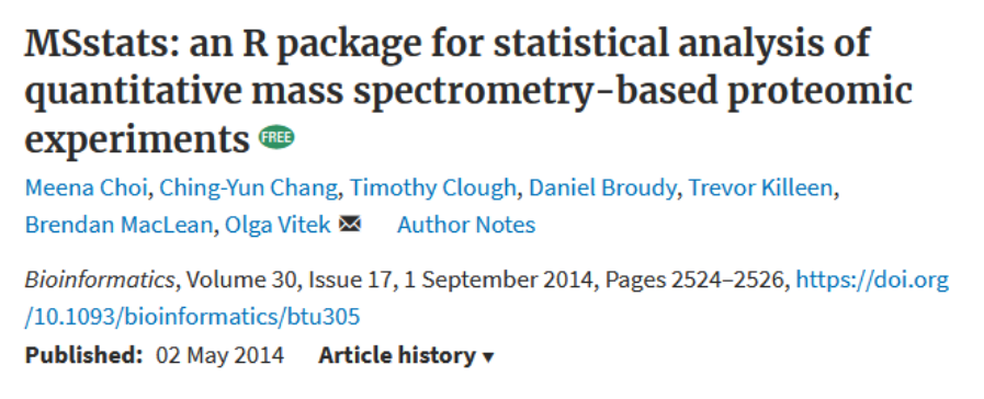
MSstats Software
.left-column50[
.image-100[
 ]
]
- Two Bioconductor R Packages
- MSstats & MSstatsTMT
- Popular open-source statistical proteomics software ]
.right-column50[
- Import and pre-process results from common proteomics software:
- MaxQuant, Skyline, OpenMS
- data processing
- Statistical modelling
- linear models to detect differentially abundant proteins in label-free and isobaric labeled experiments
]
.footnote[ Watch: MSstats videos on YouTube ]
Speaker Notes
MSstats is an open-source software for statistical modelling of quantitative proteomics data. It is compatible with complex designs of label-free and isobaric labeled quantification experiments. First several processing steps are performed. Then MSstats applies flexible linear models to detect differentially abundant proteins.
Statistical Analysis with MSstats
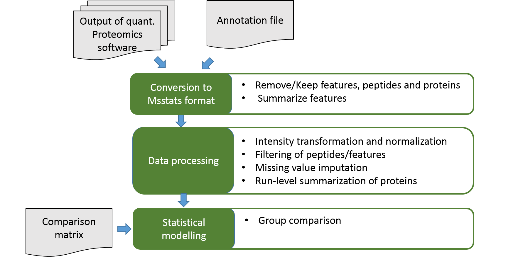
Speaker Notes
MSstats takes identified and quantified spectral peaks from common proteomics software such as MaxQuant as input. For DDA data MSstats starts with peptide level data. It applies several feature selection and processing steps in order to account for proteomics specific data properties. Afterwards MSstats calculates new protein abundances and performs statistical modelling on them.
Annotation file with experimental design
| Raw.file | Condition | BioReplicate | Run | IsotopeLabelType |
| File1.raw.thermo | Cond1 | 1 | 1 | L |
| File2.raw.thermo | Cond1 | 2 | 2 | L |
| File3.raw.thermo | Cond1 | 3 | 3 | L |
| File4.raw.thermo | Cond2 | 4 | 4 | L |
| File5.raw.thermo | Cond2 | 5 | 5 | L |
Speaker Notes
In addition to the results of the proteomics software an annotation file is needed as input. In this file the experimental design is described. It specifies conditions and biological and technical replicates. In case MaxQuant results are used as MSstats input, an additional column with the label type is needed. In a DDA experiment the value is L for all conditions.
Conversion from MaxQuant to MSstats format
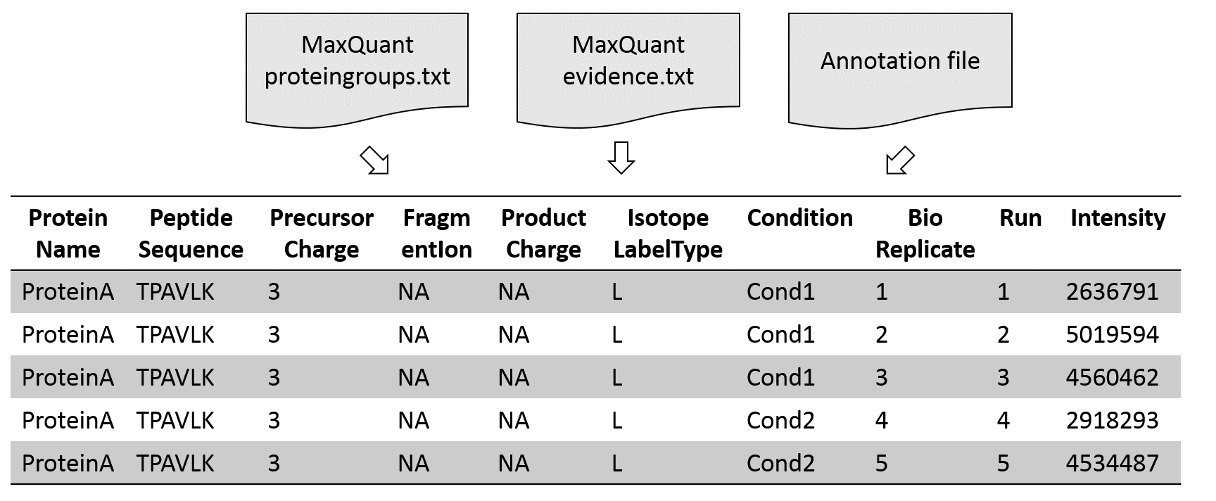
Speaker Notes
First, the input data is converted into an MSstats compatible table. For this step several parameters to filter and adjust the input data can be selected.
Intensity manipulations
- Log-transformation: log2 or log10
- Intensity normalization: equalize medians or quantile normalization
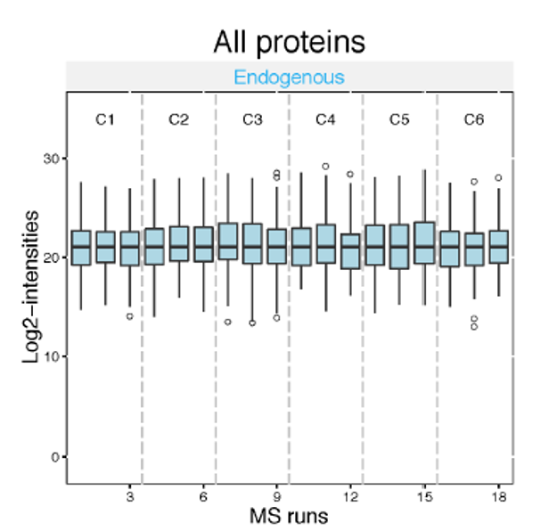
Speaker Notes
Log transformation brings the peptide intensities into a close to normal distribution. Normalization aims to make the intensities of different runs more comparable to each other. The default normalization method is called ‘equalize medians’. It assumes that the majority of proteins do not change across runs. It shifts all intensities of a run by a constant to obtain equal median intensities across runs.
Peptide filtering and missing value imputation
- Feature selection: which peptides should be kept for protein quantification
- Missing value imputation: Imputation of NA and very low abundant intensities
- Protein summarization: calculates new protein abundances after data processing via TMP model
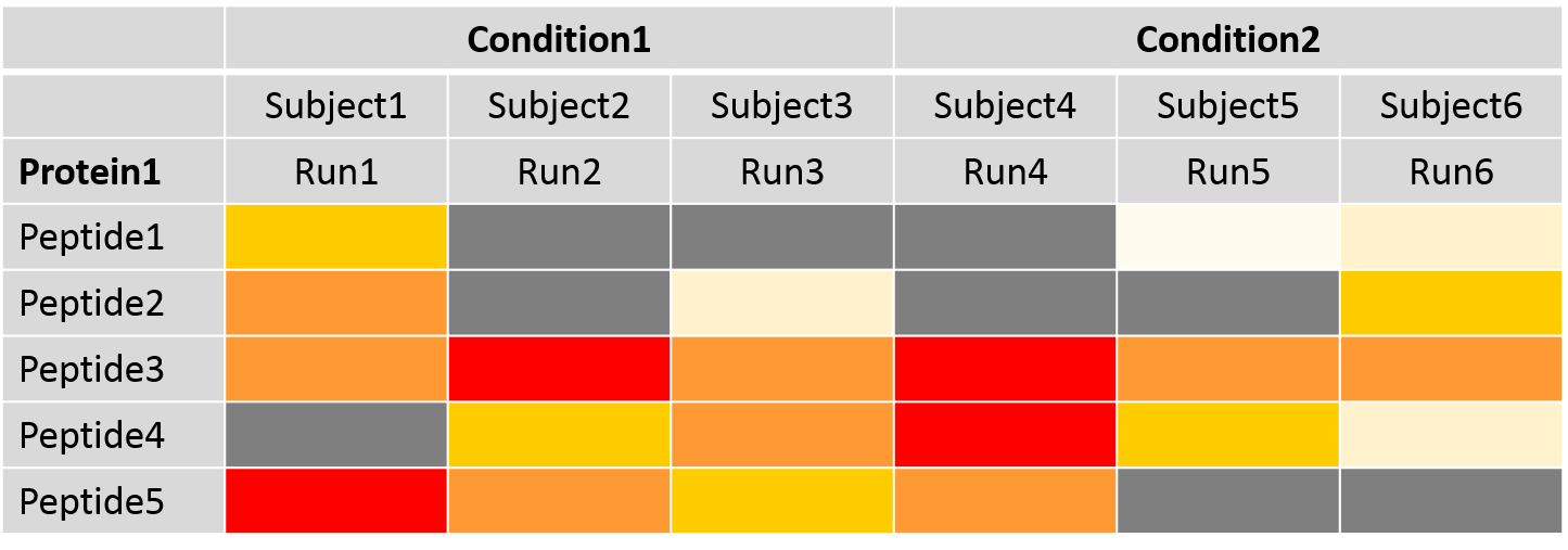
Speaker Notes
Feature selection allows the use of either all or only the most abundant peptides for protein summarization. The table represents the intensity values for the peptides of one protein. The dark grey fields represent missing intensity values of peptides. Missing values and noisy peptides with outliers are typical in label-free DDA datasets but influence protein summarization. For a reliable and robust statistical analysis, missing value imputation is recommended. Missing values in MaxQuant mean that they are missing because they were below the limit of detection. This means the values are not missing for random but for the reason of low abundance. Therefore, the values are only partially known and called “censored values”. This may also be the case for very low intensity values, which might not be reliable and can be imputed. Censored intensity values are imputed via an accelerated failure time model. Alternatively, they may be replaced with a value obtained from the other measured intensities for the peptide and/or the run. Protein summarization is by default performed via Tukey’s median polish for robust parameter estimation with median across rows and columns.
Statistical modelling
- Uses run-level summarized data for hypothesis testing
- Needs comparison matrix to specify comparisons
- Adjusts the linear model according to information from annotation file
.pull-left[ | | | | | | |:-:|:-:|:-:|:-:|:-:| | name | Cond1 | Cond2 | Cond3 | Cond4 | | cond1-cond3 | 1 | 0 | -1 | 0 | | cond1-cond4 | 1 | 0 | 0 | -1 | | cond2-cond3 | 0 | 1 | -1 | 0 | | cond2-cond4 | 0 | 1 | 0 | -1 | ]
.pull-right[
.image-100[
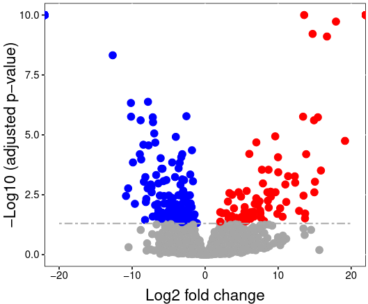 ]
]
]
]
Speaker Notes
The calculated run-level protein summaries are used for statistical group comparison. Any two conditions can be compared to find differentially abundant proteins between them. MSstats uses a family of linear mixed models for this. The model is automatically adjusted for the comparison type according to the information in the annotation file. This means MSstats accounts for technical replicates, paired designs or time course experiments automatically.
Thank you!
This material is the result of a collaborative work. Thanks to the Galaxy Training Network and all the contributors! Tutorial Content is licensed under
Creative Commons Attribution 4.0 International License.
Tutorial Content is licensed under
Creative Commons Attribution 4.0 International License.