Learning with RMarkdown in RStudio


Learning with RMarkdown is a bit different than you might be used to. Instead of copying and pasting code from the GTN into a document you’ll instead be able to run the code directly as it was written, inside RStudio! You can now focus just on the code and reading within RStudio.

  1. Load the notebook if you have not already, following the tip box at the top of the tutorial

    Screenshot of the Console in RStudio. There are three lines visible of not-yet-run R code with the download.file statements which were included in the setup tip box.

  2. Open it by clicking on the .Rmd file in the file browser (bottom right)

    Screenshot of Files tab in RStudio, here there are three files listed, a data-science-r-dplyr.Rmd file, a css and a bib file.

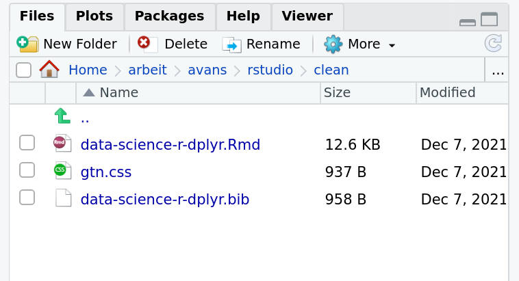
  3. The RMarkdown document will appear in the document viewer (top left)

    Screenshot of an open document in RStudio. There is some yaml metadata above the tutorial showing the title of the tutorial.

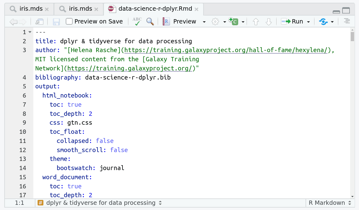
You’re now ready to view the RMarkdown notebook! Each notebook starts with a lot of metadata about how to build the notebook for viewing, but you can ignore this for now and scroll down to the content of the tutorial.

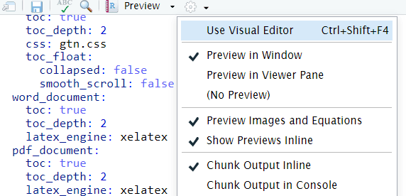
You can switch to the visual mode which is way easier to read - just click on the gear icon and select Use Visual Editor.

Screenshot of dropdown menu after clicking on the gear icon. The first option is `Use Visual Editor`.

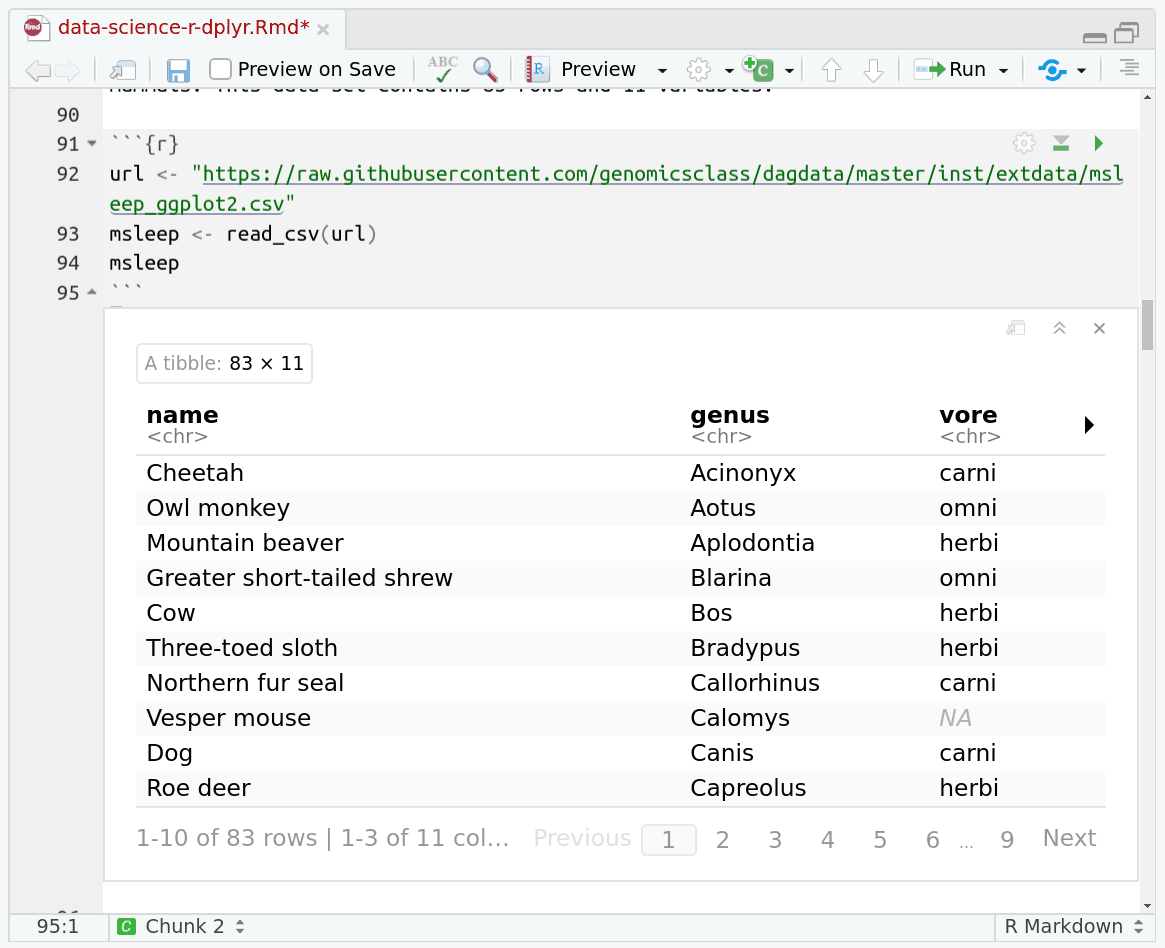
You’ll see codeblocks scattered throughout the text, and these are all runnable snippets that appear like this in the document:

Screenshot of the RMarkdown document in the viewer, a cell is visible between markdown text reading library tidyverse. It is slightly more grey than the background region, and it has a run button at the right of the cell in a contextual menu.

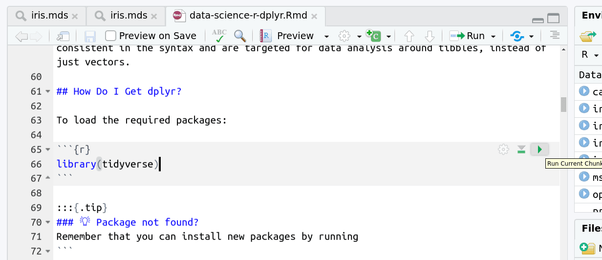
And you have a few options for how to run them:

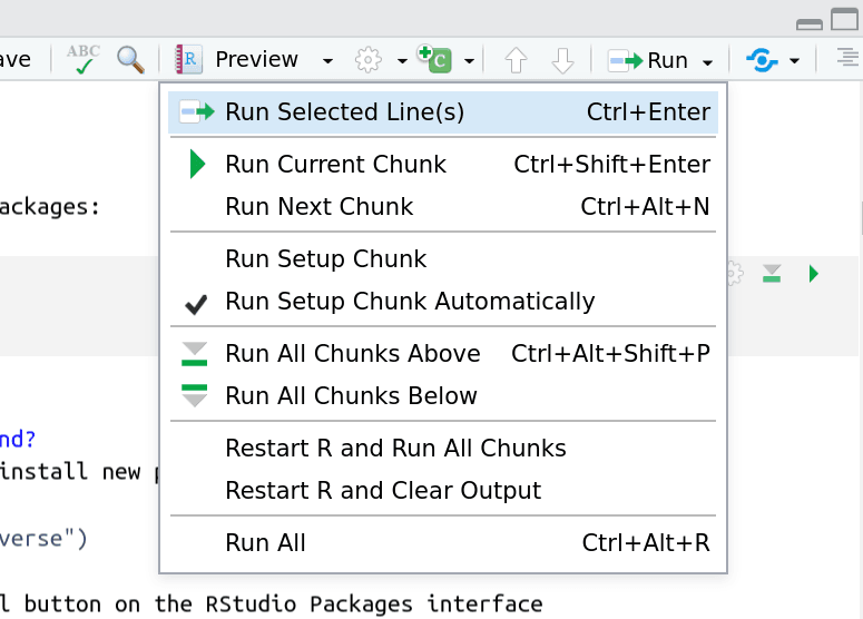
  1. Click the green arrow
  2. ctrl+enter
  3. Using the menu at the top to run all

    Screenshot of the run dropdown menu in R, the first item is run selected lines showing the mentioned shortcut above, the second is run next chunk, and then it also mentions a 'run all chunks below' and 'restart r and run all chunks' option.

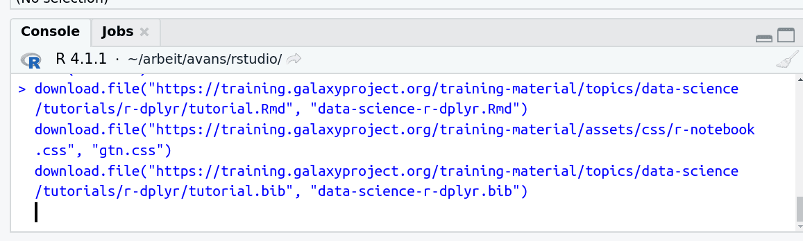
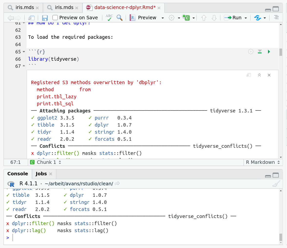
When you run cells, the output will appear below in the Console. RStudio essentially copies the code from the RMarkdown document, to the console, and runs it, just as if you had typed it out yourself!

Screenshot of a run cell, its output is included below in the RMarkdown document and the same output is visible below in the console. It shows a log of loading the tidyverse library.

One of the best features of RMarkdown documents is that they include a very nice table browser which makes previewing results a lot easier! Instead of needing to use head every time to preview the result, you get an interactive table browser for any step which outputs a table.

Screenshot of the table browser. Below a code chunk is a large white area with two images, the first reading 'r console' and the second reading 'tbl_df'. The tbl_df is highlighted like it is active. Below that is a pretty-printed table with bold column headers like name and genus and so on. At the right of the table is a small arrow indicating you can switch to seeing more columns than just the initial three. At the bottom of the table is 1-10 of 83 rows written, and buttons for switching between each page of results.

Still have questions?
Gitter Chat Support
Galaxy Help Forum
Want to embed this snippet (FAQ) in your GTN Tutorial?
{% snippet  faqs/galaxy/interactive_tools_rstudio_rmarkdown.md %}
Persistent URL
Resource purlPURL: https://gxy.io/GTN:F00084