Visualization of RNA-Seq results with Volcano Plot
| Author(s) |
|
| Editor(s) |
|
| Reviewers |
|
OverviewQuestions:
Objectives:
How to generate a volcano plot from RNA-seq data?
Requirements:
Create a volcano plot of RNA-seq data to visualize significant genes
- Introduction to Galaxy Analyses
- slides Slides: Quality Control
- tutorial Hands-on: Quality Control
- slides Slides: Mapping
- tutorial Hands-on: Mapping
- tutorial Hands-on: 2: RNA-seq counts to genes
Time estimation: 30 minutesLevel: Introductory IntroductorySupporting Materials:
- Datasets
- Workflows
- galaxy-history-answer Answer Histories
- FAQs
- video Recordings
- instances Available on these Galaxies
Published: Dec 31, 2018Last modification: Apr 17, 2025License: Tutorial Content is licensed under Creative Commons Attribution 4.0 International License. The GTN Framework is licensed under MITpurl PURL: https://gxy.io/GTN:T00304rating Rating: 4.4 (5 recent ratings, 78 all time)version Revision: 16
 Volcano plots are commonly used to display the results of RNA-seq or other omics experiments. A volcano plot is a type of scatterplot that shows statistical significance (P value) versus magnitude of change (fold change). It enables quick visual identification of genes with large fold changes that are also statistically significant. These may be the most biologically significant genes. In a volcano plot, the most upregulated genes are towards the right, the most downregulated genes are towards the left, and the most statistically significant genes are towards the top.
To generate a volcano plot of RNA-seq results, we need a file of differentially expressed results which is provided for you here. To generate this file yourself, see the RNA-seq counts to genes tutorial. The file used here was generated from limma-voom but you could use a file from any RNA-seq differential expression tool, such as edgeR or DESeq2, as long as it has the required columns (see below).
The data for this tutorial comes from Fu et al. 2015. This study examined the expression profiles of basal and luminal cells in the mammary gland of virgin, pregnant and lactating mice. Here, we will visualize the results of the luminal pregnant vs lactating comparison.
AgendaIn this tutorial, we will deal with:
Preparing the inputs
We will use two files for this analysis:
- Differentially expressed results file (genes in rows, and 4 required columns: raw P values, adjusted P values (FDR), log fold change and gene labels)
- Genes of interest file (list of genes to be plotted in volcano)
Import data
Hands On: Data upload
Create a new history for this RNA-seq exercise e.g.
Volcano plotTo create a new history simply click the new-history icon at the top of the history panel:
- Click on galaxy-pencil (Edit) next to the history name (which by default is “Unnamed history”)
- Type the new name
- Click on Save
- To cancel renaming, click the galaxy-undo “Cancel” button
If you do not have the galaxy-pencil (Edit) next to the history name (which can be the case if you are using an older version of Galaxy) do the following:
- Click on Unnamed history (or the current name of the history) (Click to rename history) at the top of your history panel
- Type the new name
- Press Enter
Import the result table of differential gene expression analysis, as well as a list of genes that will be annotated in the volcano plot later.
To import the file, there are two options:
- Option 1: From a shared data library if available (ask your instructor)
- Option 2: From Zenodo
- Copy the link location
Click galaxy-upload Upload at the top of the activity panel
- Select galaxy-wf-edit Paste/Fetch Data
Paste the link(s) into the text field
Press Start
- Close the window
As an alternative to uploading the data from a URL or your computer, the files may also have been made available from a shared data library:
- Go into Libraries (left panel)
- Navigate to the correct folder as indicated by your instructor.
- On most Galaxies tutorial data will be provided in a folder named GTN - Material –> Topic Name -> Tutorial Name.
- Select the desired files
- Click on Add to History galaxy-dropdown near the top and select as Datasets from the dropdown menu
In the pop-up window, choose
- “Select history”: the history you want to import the data to (or create a new one)
- Click on Import
You can paste the links below into the Paste/Fetch box:
https://zenodo.org/record/2529117/files/limma-voom_luminalpregnant-luminallactate
https://zenodo.org/record/2529117/files/volcano_genes
Select “Type (set all)”:
tabularAfter the files import, check that the datatype is
tabular. If the datatype is nottabular, please change the file type totabular.
- Click on the galaxy-pencil pencil icon for the dataset to edit its attributes
- In the central panel, click galaxy-chart-select-data Datatypes tab on the top
- In the galaxy-chart-select-data Assign Datatype, select
tabularfrom “New Type” dropdown
- Tip: you can start typing the datatype into the field to filter the dropdown menu
- Click the Save button


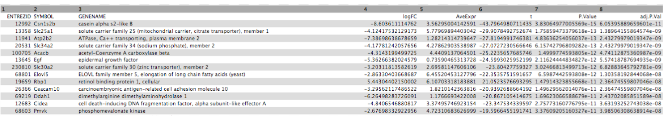
Click on the galaxy-eye (eye) icon and take a look at the limma-voom_luminalpregnant-luminallactate file. It should look like below, with 8 columns.
Create volcano plot highlighting significant genes
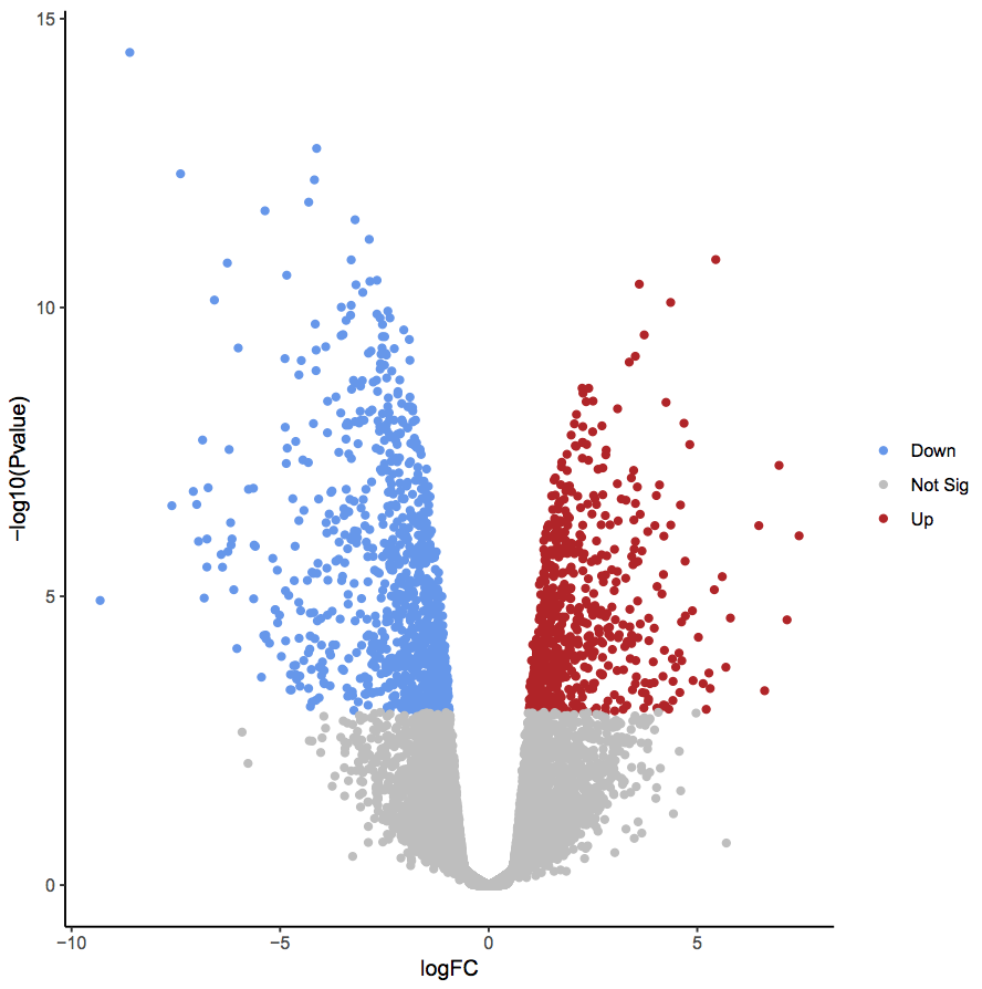
First, we will create a volcano plot highlighting all significant genes. We will call genes significant, if they have FDR < 0.01 and a log fold change of 0.58 (equivalent to a fold-change of 1.5). These were the values used in the original paper for this dataset.
Hands On: Create a Volcano plot
- Volcano Plot ( Galaxy version 0.0.7) to create a volcano plot:
- “Specify an input file”: limma-voom file
- “FDR (adjusted P value)”:
Column 8- “P value (raw)”:
Column 7- “Log Fold Change”:
Column 4- “Labels”:
Column 2- “Significance threshold”:
0.01- “LogFC threshold to colour”:
0.58- “Points to label”:
None
In the plot above the genes are coloured if they pass the thresholds for FDR and Log Fold Change. The red dots are upregulated genes and the blue dots are downregulated genes. You can see in this plot that there are many (hundreds) of significant genes in this dataset.
QuestionWhy does the y axis use a negative P value scale?
The negative log of the P values are used for the y axis so that the smallest P values (most significant) are at the top of the plot.
Create volcano plot labelling top significant genes
You can also choose to show the labels (e.g. Gene Symbols) for the significant genes with the volcano plot tool. You can select to label all significant or just the top genes. The top genes are those that pass the FDR and logFC thresholds that have the smallest P values. As there are hundreds of significant genes here, too many to sensibly label, let’s label the top 10 significant genes.
Hands On: Create a Volcano plot labelling top 10 significant genes
- Use the Run Job Again galaxy-refresh button in the History to re-run Volcano Plot ( Galaxy version 0.0.7) with the same parameters as before except:
- “Points to label”:
Significant
- “Only label top most significant”:
10
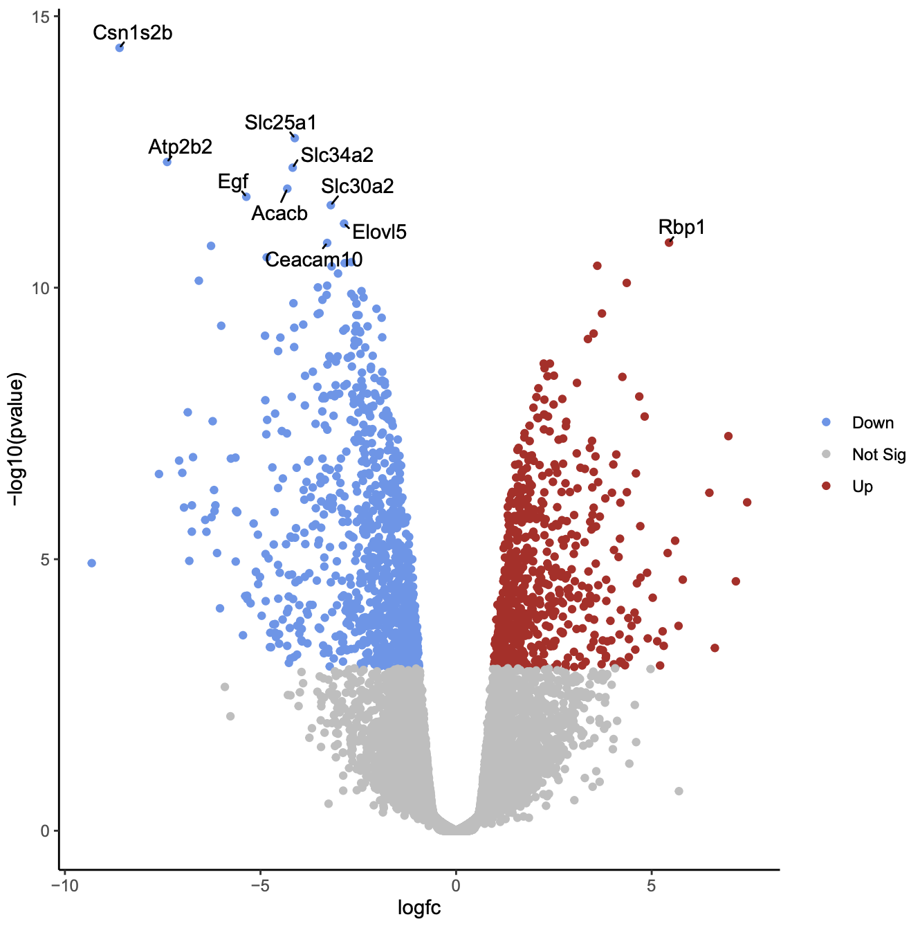
As in the previous plot, genes are coloured if they pass the thresholds for FDR and Log Fold Change, (red for upregulated and blue for downregulated) and the top genes by P value are labelled. Note that in the plot above we can now easily see what the top genes are by P value and also which of them have bigger fold changes.
QuestionWhich gene is the most statistically significant with large fold change?
Csn1s2b, as it is the gene nearest the top of the plot and it is also far to the left. This gene is a calcium-sensitive casein that is important in milk production. As this dataset compares lactating and pregnant mice, it makes sense that it is a gene that is very differentially expressed.
Create volcano plot labelling genes of interest
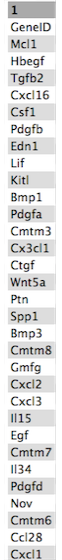
We can also label one or more genes of interest in a volcano plot. This enables us to visualize where these genes are in terms of significance and in comparison to the other genes. In the original paper using this dataset, there is a heatmap of 31 genes in Figure 6b (have a look at this visualization tutorial if you would like to see how to generate the heatmap). These genes are a set of 30 cytokines/growth factor identified as differentially expressed, and the authors’ main gene of interest, Mcl1. These genes are provided in the volcano_genes file and shown below. We will label these genes in the volcano plot. We’ll add boxes around the labels to highlight the gene names.
Hands On: Create a Volcano plot labelling genes of interest
- Use the Run Job Again galaxy-refresh button in the History to re-run Volcano Plot ( Galaxy version 0.0.7) with the same parameters as before except:
- “Points to label”:
Input from file
- “File of labels”:
volcano_genes- In “Plot Options”:
- “Label Boxes”:
Yes
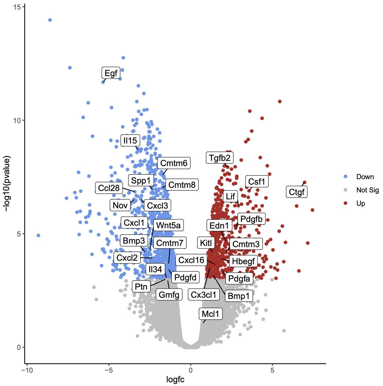
Question
- How many of the genes of interest are significant?
Which gene of interest is the most statistically significant?
- 29/31 are significant, the genes that are not in the grey area.
- The Egf gene is the most statistically significant as it is nearest the top of the plot.
As in the previous plots, genes are coloured if they pass the thresholds for FDR and Log Fold Change. Here, all the genes of interest are significant (red or blue) except for two genes, Mcl1 and Gmfg. Gmfg, has an FDR just very slightly outside the significance threshold we used of 0.01 (0.0105). Mcl1 is the authors’ gene of interest and they showed that while it’s expression did increase at the protein level, it did not increase at the transcription level, as we can see here, suggesting it is regulated post-transcriptionally.
You can get the R code used to generate the plot under Output Options in the tool form. You can edit this code in R if you want to customise the plot. See the Visualization of RNA-Seq results with Volcano Plot in R tutorial for how to do this.
Conclusion
In this tutorial we have seen how a volcano plot can be generated from RNA-seq data and used to quickly visualize significant genes.
You've Finished the Tutorial
Key points
A volcano plot can be used to quickly visualize significant genes in RNA-seq results
Frequently Asked Questions
Have questions about this tutorial? Have a look at the available FAQ pages and support channelsUseful literature
Further information, including links to documentation and original publications, regarding the tools, analysis techniques and the interpretation of results described in this tutorial can be found here.
References
- Fu, N. Y., A. C. Rios, B. Pal, R. Soetanto, A. T. L. Lun et al., 2015 EGF-mediated induction of Mcl-1 at the switch to lactation is essential for alveolar cell survival. Nature Cell Biology 17: 365–375. 10.1038/ncb3117
Feedback
Did you use this material as an instructor? Feel free to give us feedback on how it went.
Did you use this material as a learner or student? Click the form below to leave feedback.

Citing this Tutorial
- Maria Doyle, Visualization of RNA-Seq results with Volcano Plot (Galaxy Training Materials). https://training.galaxyproject.org/training-material/topics/transcriptomics/tutorials/rna-seq-viz-with-volcanoplot/tutorial.html Online; accessed TODAY
- Hiltemann, Saskia, Rasche, Helena et al., 2023 Galaxy Training: A Powerful Framework for Teaching! PLOS Computational Biology 10.1371/journal.pcbi.1010752
- Batut et al., 2018 Community-Driven Data Analysis Training for Biology Cell Systems 10.1016/j.cels.2018.05.012
Congratulations on successfully completing this tutorial!@misc{transcriptomics-rna-seq-viz-with-volcanoplot, author = "Maria Doyle", title = "Visualization of RNA-Seq results with Volcano Plot (Galaxy Training Materials)", year = "", month = "", day = "", url = "\url{https://training.galaxyproject.org/training-material/topics/transcriptomics/tutorials/rna-seq-viz-with-volcanoplot/tutorial.html}", note = "[Online; accessed TODAY]" } @article{Hiltemann_2023, doi = {10.1371/journal.pcbi.1010752}, url = {https://doi.org/10.1371%2Fjournal.pcbi.1010752}, year = 2023, month = {jan}, publisher = {Public Library of Science ({PLoS})}, volume = {19}, number = {1}, pages = {e1010752}, author = {Saskia Hiltemann and Helena Rasche and Simon Gladman and Hans-Rudolf Hotz and Delphine Larivi{\`{e}}re and Daniel Blankenberg and Pratik D. Jagtap and Thomas Wollmann and Anthony Bretaudeau and Nadia Gou{\'{e}} and Timothy J. Griffin and Coline Royaux and Yvan Le Bras and Subina Mehta and Anna Syme and Frederik Coppens and Bert Droesbeke and Nicola Soranzo and Wendi Bacon and Fotis Psomopoulos and Crist{\'{o}}bal Gallardo-Alba and John Davis and Melanie Christine Föll and Matthias Fahrner and Maria A. Doyle and Beatriz Serrano-Solano and Anne Claire Fouilloux and Peter van Heusden and Wolfgang Maier and Dave Clements and Florian Heyl and Björn Grüning and B{\'{e}}r{\'{e}}nice Batut and}, editor = {Francis Ouellette}, title = {Galaxy Training: A powerful framework for teaching!}, journal = {PLoS Comput Biol} }
Do you want to extend your knowledge?Follow one of our recommended follow-up trainings:
You can use Ephemeris's
shed-tools installcommand to install the tools used in this tutorial.shed-tools install [-g GALAXY] [-a API_KEY] -t <(curl https://training.galaxyproject.org/training-material/api/topics/transcriptomics/tutorials/rna-seq-viz-with-volcanoplot/tutorial.json | jq .admin_install_yaml -r)Alternatively you can copy and paste the following YAML
---
install_tool_dependencies: true
install_repository_dependencies: true
install_resolver_dependencies: true
tools:
- name: volcanoplot
  owner: iuc
  revisions: 5e08a1e22dbc
  tool_panel_section_label: Graph/Display Data
  tool_shed_url: https://toolshed.g2.bx.psu.edu/