The practical aims at familiarzing you with Climate Science and the terminology used by climate scientists. The target audience is not a climate scientist but
anyone interested in learning about climate.
European Copernicus Climate Change Service (C3S) provide authoritative information about the past, present
and future climate. C3S is one of the many services provided by Copernicus, the European Union’s Earth Observation Programme, looking
at our planet and its environment for the ultimate benefit of all European citizens.
The C3S Climate Data Store (CDS) provides a single point of access to a wide range of
quality-assured climate datasets distributed in the cloud.
Access to data from the CDS is open and unrestricted. While registration is required, it is free of charge.
We will be using freely available datasets from the CDS, including
observations, historical climate data records, estimates of Essential Climate Variables (ECVs) derived from Earth observations,
global and regional climate reanalyses of past observations, seasonal forecasts and climate projections. To make access easier and faster,
the datasets have been prepared and deposited on Zenodo. At the end of the tutorial, feel free to visit the CDS to download alternative
datasets.
For the purpose of this tutorial, sample datasets have been created from data downloaded from C3S through
Copernicus Climate Data Store:
To reduce the volume of data, the data resolution (in space and/or time) has been significantly reduced and/or data has been selected on sample locations (Paris, Oslo and
Freiburg). The data format may also have been changed (for instance to tabular) to ease processing.
Get data
Hands On: Data upload
Create a new history for this tutorial. If you are not inspired, you can name it climate101.
To create a new history simply click the new-history icon at the top of the history panel:
Import the files from Zenodo or from the shared data library
Click galaxy-uploadUpload at the top of the activity panel
Select galaxy-wf-editPaste/Fetch Data
Paste the link(s) into the text field
Press Start
Close the window
As an alternative to uploading the data from a URL or your computer, the files may also have been made available from a shared data library:
Go into Libraries (left panel)
Navigate to the correct folder as indicated by your instructor.
On most Galaxies tutorial data will be provided in a folder named GTN - Material –> Topic Name -> Tutorial Name.
Select the desired files
Click on Add to Historygalaxy-dropdown near the top and select as Datasets from the dropdown menu
In the pop-up window, choose
“Select history”: the history you want to import the data to (or create a new one)
Click on Import
Check that the datatype is tabular
Click on the galaxy-pencilpencil icon for the dataset to edit its attributes
In the central panel, click galaxy-chart-select-dataDatatypes tab on the top
In the galaxy-chart-select-dataAssign Datatype, select datatypes from “New Type” dropdown
Tip: you can start typing the datatype into the field to filter the dropdown menu
Click the Save button
If it is not tabular make sure to convert it using the Galaxy built-in format converters.
Click on the galaxy-pencil pencil icon for the dataset to edit its attributes.
In the central panel, click galaxy-chart-select-data Datatypes tab on the top.
In the galaxy-gear Convert to Datatype section, select Convert CSV to Tabular from “Target datatype” dropdown.
Click the Create Dataset button to start the conversion.
Rename Datasets
As “https://zenodo.org/record/3776500/files/tg_ens_mean_0.1deg_reg_v20.0e_Paris_daily.csv” is not a beautiful name and can give errors for some tools, it is a good practice to change the dataset name by something more meaningful.
For example by removing https://zenodo.org/record/3776500/files/ to obtain tg_ens_mean_0.1deg_reg_v20.0e_Paris_daily.csv and ts_cities.csv, respectively.
Click on the galaxy-pencilpencil icon for the dataset to edit its attributes
In the central panel, change the Name field
Click the Save button
Add a tag to the dataset corresponding to copernicus
Datasets can be tagged. This simplifies the tracking of datasets across the Galaxy interface. Tags can contain any combination of letters or numbers but cannot contain spaces.
To tag a dataset:
Click on the dataset to expand it
Click on Add Tagsgalaxy-tags
Add tag text. Tags starting with # will be automatically propagated to the outputs of tools using this dataset (see below).
Press Enter
Check that the tag appears below the dataset name
Tags beginning with # are special!
They are called Name tags. The unique feature of these tags is that they propagate: if a dataset is labelled with a name tag, all derivatives (children) of this dataset will automatically inherit this tag (see below). The figure below explains why this is so useful. Consider the following analysis (numbers in parenthesis correspond to dataset numbers in the figure below):
a set of forward and reverse reads (datasets 1 and 2) is mapped against a reference using Bowtie2 generating dataset 3;
dataset 3 is used to calculate read coverage using BedTools Genome Coverageseparately for + and - strands. This generates two datasets (4 and 5 for plus and minus, respectively);
datasets 4 and 5 are used as inputs to Macs2 broadCall datasets generating datasets 6 and 8;
datasets 6 and 8 are intersected with coordinates of genes (dataset 9) using BedTools Intersect generating datasets 10 and 11.
Now consider that this analysis is done without name tags. This is shown on the left side of the figure. It is hard to trace which datasets contain “plus” data versus “minus” data. For example, does dataset 10 contain “plus” data or “minus” data? Probably “minus” but are you sure? In the case of a small history like the one shown here, it is possible to trace this manually but as the size of a history grows it will become very challenging.
The right side of the figure shows exactly the same analysis, but using name tags. When the analysis was conducted datasets 4 and 5 were tagged with #plus and #minus, respectively. When they were used as inputs to Macs2 resulting datasets 6 and 8 automatically inherited them and so on… As a result it is straightforward to trace both branches (plus and minus) of this analysis.
According to wikipedia,
Climate is defined as the average state of everyday’s weather condition over a period of 30 years. It is measured by assessing
the patterns of variation in temperature, humidity, atmospheric pressure, wind, precipitation, atmospheric particle count and
other meteorological variables in a given region over a long period of time (usually 20 or 30 years).
Climate differs from weather, in that weather only describes the short-term conditions of these variables in a given region.
Climate versus Weather
Quantities that climate scientists are interested in are similar to those used to assess the weather (temperature, precipitation, etc.).
But there is a big difference between climate and weather: weather varies from hour to hour and from day to day whereas climate
is defined as the average of weather over several decades or longer.
The figure below shows a woman walking her dog and we can use it to make an analogy to illustrate the difference between weather and climate.
if you focus your attention on the dog, you can see that it is all over the place, sometimes upwards, sometimes downwards: this can represent the weather and its
variability. The dog (weather) is not following a fully random pattern and varies around a main direction (trend) that is given by the woman: the woman is representing
the climate and gives us an indication of where both the woman and dog are likely to be in the future.
You can also watch an animated illustration of the difference between climate and weather:
Video: Difference between climate and weather
What is the weather like in Paris?
In order to answer this question, we are going to inspect and visualize the dataset tg_ens_mean_0.1deg_reg_v20.0e_Paris_daily.csv using simple galaxy tools.
Hands On: Daily temperature time series
Comment: Tip: search for the tool
Many different tools can be used to answer to the questions. Here we give you some guidelines to help you to choose.
Use the tools search box at the top of the tool panel to find Select lines that match an expressiontool and Datamashtool.
Question
What was the average temperature in Paris on the 14th of July 2003?
What is the minimum and maximum temperatures in Paris?
On which date did the minimum temperature occured?
On which date did the maximum temperature occured?
The average temperature in Paris on the 14th of July 2003 was 26.73 degrees Celcius. It can be found by using Select lines that match an expressiontool with parameter “the pattern” set to 2003-07-14.
The minimum temperature in Paris is -11.6799995 degrees celcius and the maximum temperature in Paris is 33.579998 degrees celcius. To find out, you can use Datamashtool with the following parameters:
param-repeat“Insert Operation to perform on each group”
“Type”: minimum
“On column”: c2
param-repeat“Insert Operation to perform on each group”
“Type”: maximum
“On column”: c2
The minimum temperature (-11.6799995 degrees celcius) was observed on January 16 1985.
You can use different Galaxy tools to find out the solution and here we show you how to use Datamashtool with the following parameters:
param-repeat“Insert Operation to perform on each group”
“Type”: maximum
“On column”: c2
What is the climate in Paris?
To get some information about the (past and current) climate in Paris, we will first look at monthly averages.
Seasonality
Hands On: What is the monthly climatological temperature in Paris?
To answer to this question, we will compute the global average temperatures over the entire period 1950 and 2019 for each month (January, February, etc.). Indeed,
this period of time is sufficiently long for computing monthly climatological temperature (more than 30 years).
Question
What is the warmest summer month e.g. between June, July and August (JJA) in Paris?
What is the coolest winter month e.g. between December, January and February (DJF) in Paris?
The warmest summer month in Paris is July (19.921018171429 degrees celcius). However, it is interesting to remark that on our dataset we see very little difference in the mean temperature between July and August.
The coolest winter month in Paris is January (4.4669169722484 degrees celcius).
Below, we show you how we found these results.
We will first split all the dates (first column) from YYYY-MM-DD (where YYYY is the year, MM the month and DD the day) to three column to get 3 columns: one for the year, one for the month and one for the day. Use Text reformatting with awktool with parameters:
File to process: tg_ens_mean_0.1deg_reg_v20.0e_Paris_daily.csv
AWK Program: gsub(/-/,"\t",$1){$1=$1} {print}
Rename the resulting file to split_dates_Paris.csv.
Then use Datamashtool with the following parameters:
param-repeat“Insert Operation to perform on each group”
“Type”: maximum
“On column”: c2
The result is in the first column of the resulting file which indicates 01 e.g. January.
Please note that you may use other Galaxy tools to reach the same results.
Results can be slightly different when using different source of climate information. However, you will always observe the same pattern e.g. cool month in winter and warm month on summer. We can also clearly see that Paris has a mild climate with on average no extreme temperatures.
In this tutorial, we compute manually the monthly climatological temperatures to explain you the algorithm used behing.
However, many data providers have pre-computed climatologies and can be directly downloaded. For instance, on the CDS, climatologies are provided for Essential climate variables for assessment of climate variability from 1979 to present.
Yearly average
Hands On: What is the trend (cooling/warming) in the climate for Paris between 1950 and 2019?
To answer to this question, we will compute yearly mean of the temperature in Paris and visualize it.
param-repeat“Insert Operation to perform on each group”
- “Type”: Mean
- “On column”: c4
Rename the resulting file to yearly_mean_Paris.csv.
To make a plot, you can use Scatterplot w ggplot2tool with the following parameters:
“Input in tabular format”: yearly_mean_Paris.csv
“Column to plot on x-axis”: 1
“Column to plot on y-axis”: 2
“Plot title”: Yearly mean temperature in Paris from 1950 to 2019
“Label for x axis”: Year (YYYY)
“Label for y axis”: Temperature (degrees celcius)
And finally in Advanced Options change Type of plot to Points and Lines.
Viewgalaxy-eye the resulting plot:
Question
Can we easily observe a trend?
The plot clearly shows a slight increase in the yearly mean temperature between 1950 and 2019. Even though it looks no more than a few degrees celcius, it is
quite significant.
Anomalies
In climate change studies, temperature anomalies are more important than absolute temperature. A temperature anomaly is the difference from an average, or baseline,
temperature. The baseline temperature is typically computed by averaging 30 or more years of temperature data. A positive anomaly indicates the observed temperature was warmer than the baseline, while a negative anomaly indicates the observed temperature was cooler than the baseline.
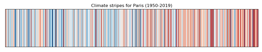
Hands On: Climate stripes for Paris
Computing temperature anomalies is out of scope of this tutorial and we will therefore use pre-computed temperature anomalies ts_cities.csv.
A simple way to visualize anomalies and highlight cooling/warming over the years, is to use climate stripes from timeseriestool with the following parameters:
“timeseries to plot”: ts_cities.csv
“column name to use for plotting”: tg_anomalies_paris
“plot title”: Climate stripes for Paris (1950-2019)
Viewgalaxy-eye the resulting plot:
Question: do you observe a warming or cooling between 1950 and 2019?
The climate stripes clearly show a warming between 1950 and 2019.
Copernicus Climate Bulletins presents the current condition of the climate using key climate change indicators.
They also provide data, analysis of the maps and guidance on how they are produced. Datasets for temperature anomalies can be found and are
regularly updated (with recent dates). For instance, in March 2020, the corresponding dataset can be found on the Copernicus site.
Climate variables
Temperature is often the first variable that comes to mind when we talk about climate. However, it is insufficient to fully characterize the climate, and scientists have agreed on a number of variables to systematically observe Earth`s changing climate.
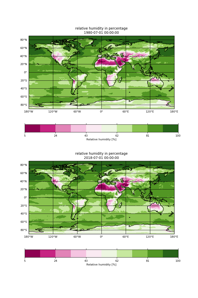
We will look at the Water Vapor Essential Climate Variable :
The humidity of air near the surface of the Earth affects the comfort and health of humans, livestock and wildlife, the swarming behaviour of insects and the occurrence of plant disease. The humidity of air near the surface affects evaporation and the strength of the hydrological and energy cycles. Evaporation from the surface of the earth is the source of water in the atmosphere and so is responsible for important feedbacks in the climate system due to clouds and radiation.
Import the file from Zenodo or from the shared data library
Currently Panoply in Galaxy is available on useGalaxy.eu instance, on the “Interactive tools” tool panel section or, as all interactive tools, from the dedicated usGalaxy.eu subdomain: Live.useGalaxy.eu
Change the Color Table (Scale Tab) to “tokyo.cpt”, and
Change the Projection (Map Tab) to “Equirectangular (Regional) and the center latitude to “45” North to zoom over France.
Switch between 1980 and 2018 in the ‘Array(s)’ tab to observe the changes between these two years.
Question: Relative humidity
Do you observe any significant changes relative humidity in France from 1979 to 2018?
Do we have sufficient information to make any conclusions on the change in climate?
We can see significant changes on the plot over France. The relative humidity of air near the surface of the Earth is lower in July 2018 than in July 1980.
We do not have sufficient information to draw any conclusions about the change in climate. In our analysis, we only used two different months (July 1980 and July 2018) and can only discuss the average changes in weather during these two periods (July 1980 and July 2018). We learnt that to draw any conclusions on the climate, we would need to make statistics over a long period of time e.g. we would need to download about 30 years of data and for instance compute anomalies in relative humidity to check if there is any trend. These aspects will be discussed further in other Galaxy tutorials.
Past, present and future climate?
When we talk about climate data, the type of data can vary significantly. We have very little actual observations at the scale of climate and usually not covering a large area. In addition to observations, we can make use of:
Re-analyses where observations and numerical modelling are combined together.
Climate models.
Observations and re-analyses provide information about the past and current climate while climate models can provide past, current and future climate information.
When it comes to future climate, we usually need to make some assumptions (such as how much CO2 emissions, etc.) and simulate different scenarios e.g. we run climate models using different assumptions and look at future trends under each of these scenarios: this is what we call climate projections. Climate projections will be discussed in a separate Galaxy tutorial.
Conclusion
We have learnt to differentiate climate from weather and got an overview of the terminology used by climate scientists to identify the
various source of climate data.
You've Finished the Tutorial
Please also consider filling out the Feedback Form as well!
Key points
Weather versus Climate
Essential Climate Variables
Observations, reanalysis, predictions and projections.
Frequently Asked Questions
Have questions about this tutorial? Have a look at the available FAQ pages and support channels
Did you use this material as an instructor? Feel free to give us feedback on how it went.
Did you use this material as a learner or student? Click the form below to leave feedback.
Hiltemann, Saskia, Rasche, Helena et al., 2023 Galaxy Training: A Powerful Framework for Teaching! PLOS Computational Biology 10.1371/journal.pcbi.1010752
Batut et al., 2018 Community-Driven Data Analysis Training for Biology Cell Systems 10.1016/j.cels.2018.05.012
@misc{climate-climate-101,
author = "Anne Fouilloux",
	title = "Getting your hands-on climate data (Galaxy Training Materials)",
	year = "",
	month = "",
	day = "",
	url = "\url{https://training.galaxyproject.org/training-material/topics/climate/tutorials/climate-101/tutorial.html}",
	note = "[Online; accessed TODAY]"
}
@article{Hiltemann_2023,
	doi = {10.1371/journal.pcbi.1010752},
	url = {https://doi.org/10.1371%2Fjournal.pcbi.1010752},
	year = 2023,
	month = {jan},
	publisher = {Public Library of Science ({PLoS})},
	volume = {19},
	number = {1},
	pages = {e1010752},
	author = {Saskia Hiltemann and Helena Rasche and Simon Gladman and Hans-Rudolf Hotz and Delphine Larivi{\`{e}}re and Daniel Blankenberg and Pratik D. Jagtap and Thomas Wollmann and Anthony Bretaudeau and Nadia Gou{\'{e}} and Timothy J. Griffin and Coline Royaux and Yvan Le Bras and Subina Mehta and Anna Syme and Frederik Coppens and Bert Droesbeke and Nicola Soranzo and Wendi Bacon and Fotis Psomopoulos and Crist{\'{o}}bal Gallardo-Alba and John Davis and Melanie Christine Föll and Matthias Fahrner and Maria A. Doyle and Beatriz Serrano-Solano and Anne Claire Fouilloux and Peter van Heusden and Wolfgang Maier and Dave Clements and Florian Heyl and Björn Grüning and B{\'{e}}r{\'{e}}nice Batut and},
	editor = {Francis Ouellette},
	title = {Galaxy Training: A powerful framework for teaching!},
	journal = {PLoS Comput Biol}
}
Congratulations on successfully completing this tutorial!
You can use Ephemeris's shed-tools install command to install the tools used in this tutorial.
5 stars:
Liked: Very nice intro. Learned about the difference between climate and weather!
4 stars:
Liked: Clear introduction in using galaxy to explore/map climate data.
Disliked: More detailed explanation of the inputs @map plot gridded (lat/lon) netCDF data. Did not understand the R as input “variable name as given in the netCDF file”. For other Essential Climate Variables I guess Ill have to change that input?
July 2020
5 stars:
Liked: Exposure to climate concepts and tool choices.
Questions:


 Open image in new tab
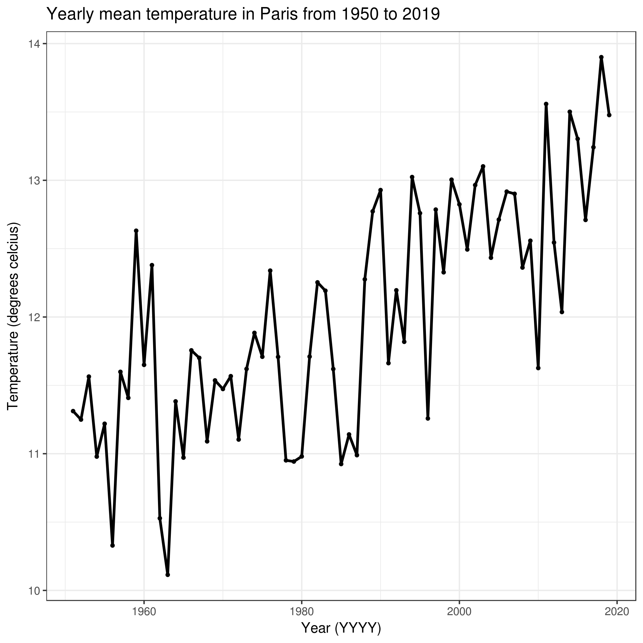
Open image in new tab