Visualization of RNA-Seq results with Volcano Plot in R
OverviewQuestions:
Objectives:
How to customise Volcano plot output in R?
Requirements:
Learn how to use R to edit Volcano plot colours, points, labels and categories
- Introduction to Galaxy Analyses
- Sequence analysis
- Hands-on: Hands-on: Quality Control: slides slides - tutorial hands-on
- Hands-on: Hands-on: Mapping: slides slides - tutorial hands-on
- Using Galaxy and Managing your Data
- RStudio in Galaxy: tutorial hands-on
- Foundations of Data Science
- R basics in Galaxy: tutorial hands-on
- Advanced R in Galaxy: tutorial hands-on
- Transcriptomics
- Visualization of RNA-Seq results with Volcano Plot: tutorial hands-on
- RNA Seq Counts to Viz in R: tutorial hands-on
Time estimation: 1 hourLevel: Intermediate IntermediateSupporting Materials:Published: Jun 14, 2021Last modification: Nov 3, 2023License: Tutorial Content is licensed under Creative Commons Attribution 4.0 International License. The GTN Framework is licensed under MITpurl PURL: https://gxy.io/GTN:T00305rating Rating: 3.0 (0 recent ratings, 4 all time)version Revision: 13
The Volcano plot tutorial, introduced volcano plots and showed how they can be generated with the Galaxy Volcano plot tool. In this tutorial we show how you can customise a plot using the R script output from the tool.
AgendaIn this tutorial, we will deal with:
Preparing the inputs
We will use one file for this analysis:
- Differentially expressed results file (genes in rows, and 4 required columns: raw P values, adjusted P values (FDR), log fold change and gene labels).
If you are following on from the Volcano plot tutorial, you already have this file in your History so you can skip to the Create volcano plot step below.
Import data
Hands-on: Data upload
Create a new history for this exercise e.g.
Volcano plot RClick the new-history icon at the top of the history panel:
- Click on galaxy-pencil (Edit) next to the history name (which by default is “Unnamed history”)
- Type the new name
- Click on Save
If you do not have the galaxy-pencil (Edit) next to the history name:
- Click on Unnamed history (or the current name of the history) (Click to rename history) at the top of your history panel
- Type the new name
- Press Enter
Import the differentially results table.
To import the file, there are two options:
- Option 1: From a shared data library if available (ask your instructor)
- Option 2: From Zenodo
- Copy the link location
Click galaxy-upload Upload Data at the top of the tool panel
- Select galaxy-wf-edit Paste/Fetch Data
Paste the link(s) into the text field
Press Start
- Close the window
As an alternative to uploading the data from a URL or your computer, the files may also have been made available from a shared data library:
- Go into Shared data (top panel) then Data libraries
- Navigate to the correct folder as indicated by your instructor.
- On most Galaxies tutorial data will be provided in a folder named GTN - Material –> Topic Name -> Tutorial Name.
- Select the desired files
- Click on Add to History galaxy-dropdown near the top and select as Datasets from the dropdown menu
In the pop-up window, choose
- “Select history”: the history you want to import the data to (or create a new one)
- Click on Import
You can paste the link below into the Paste/Fetch box:
https://zenodo.org/record/2529117/files/limma-voom_luminalpregnant-luminallactateCheck that the datatype is
tabular. If the datatype is nottabular, please change the file type totabular.
- Click on the galaxy-pencil pencil icon for the dataset to edit its attributes
- In the central panel, click galaxy-chart-select-data Datatypes tab on the top
- In the galaxy-chart-select-data Assign Datatype, select
tabularfrom “New type” dropdown
- Tip: you can start typing the datatype into the field to filter the dropdown menu
- Click the Save button

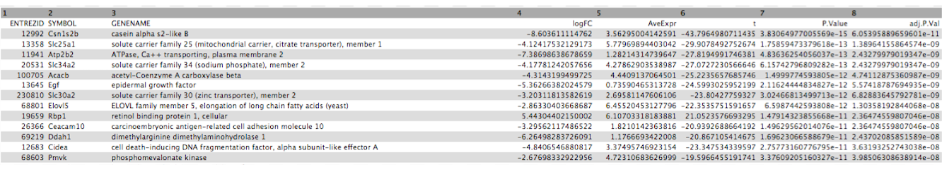
Click on the galaxy-eye (eye) icon and take a look at the DE results file. It should look like below, with 8 columns.
Create volcano plot
We will create a volcano plot colouring all significant genes. We will call genes significant here if they have FDR < 0.01 and a log2 fold change of 0.58 (equivalent to a fold-change of 1.5). These were the values used in the original paper for this dataset. We will also label the top 10 most significant genes with their gene names. We will select to output the Rscript file which we will then use to edit the plot in R.
Hands-on: Create a Volcano plot
- Volcano Plot ( Galaxy version 0.0.5) to create a volcano plot
- param-file “Specify an input file”: the de results file
- param-file “File has header?”:
Yes- param-select “FDR (adjusted P value)”:
Column 8- param-select “P value (raw)”:
Column 7- param-select “Log Fold Change”:
Column 4- param-select “Labels”:
Column 2- param-text “Significance threshold”:
0.01- param-text “LogFC threshold to colour”:
0.58- param-select “Points to label”:
Significant
- param-text “Only label top most significant”:
10- In “Output Options”:
- param-select “Output Rscript?”:
Yes
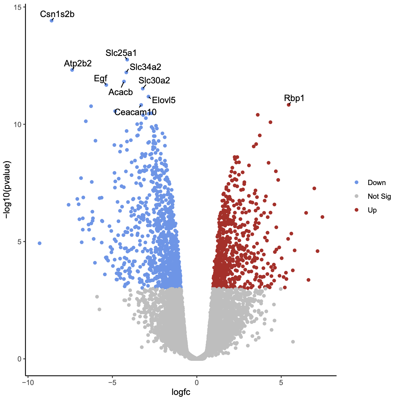
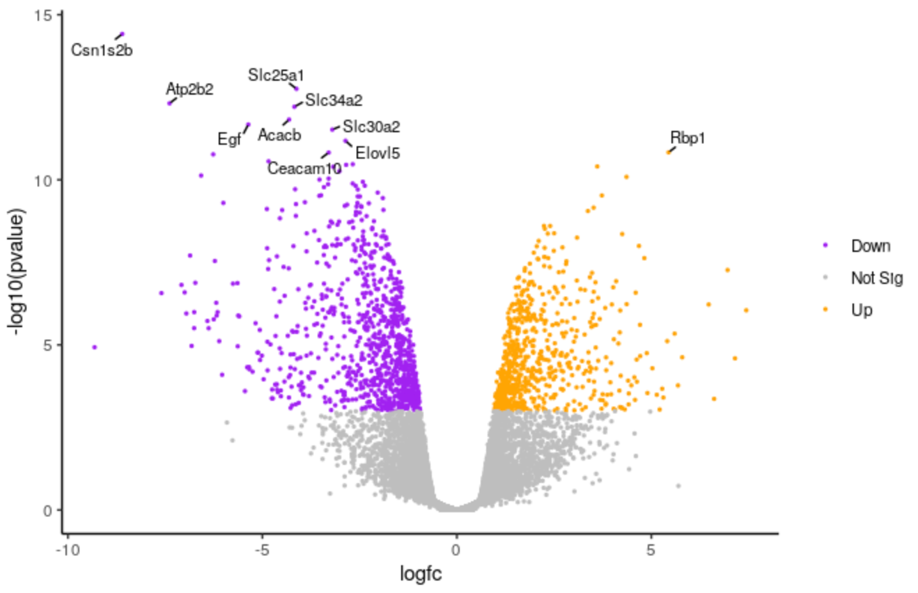
Click on the PDF file name to check that you see a plot like below.
Now we will customise the plot by editing the R code in RStudio. You can use Galaxy RStudio if available or another R such as RStudio Cloud or RStudio installed on your computer.
Import files into R
We’ll import the differentially expressed results input file and the RScript into R.
Hands-on: Using datasets from Galaxy
Note the history IDs of 1) the differentially expressed results and 2) the RScript in your Galaxy history
RStudio in Galaxy provides some special functions such as
gx_getto import and export files from your history.Hands-on: Launch RStudioDepending on which server you are using, you may be able to run RStudio directly in Galaxy. If that is not available, RStudio Cloud can be an alternative.
Currently RStudio in Galaxy is only available on UseGalaxy.eu and UseGalaxy.org
- Open the Rstudio tool tool by clicking here to launch RStudio
- Click Run Tool
- The tool will start running and will stay running permanently
- Click on the “User” menu at the top and go to “Active InteractiveTools” and locate the RStudio instance you started.
If RStudio is not available on the Galaxy instance:
- Register for RStudio Cloud, or login if you already have an account
- Create a new project
Copy the files we need into our workspace so we can see them in the Files pane.
file.copy(gx_get(1), "de-results.tsv") # will copy dataset number 1 from your history, use the correct ID for your differentially expressed results dataset.
file.copy(gx_get(3), "volcano.R") # will copy dataset number 3 from your history, use the correct ID for your Rscript dataset.
Click on
volcano.Rin the Files pane to open it in the Editor pane.
We’ll have a look at the script.
Set up script
The first few lines from # Galaxy settings start to # Galaxy settings end are settings needed to run the Volcano plot tool in Galaxy. We don’t need them to run the script in R so we will delete them. If we don’t delete the error handling line, the R session will crash if we encounter any error in the code. It’s ok as it will resume again where we were but better to not have this happen.
Hands-on: Delete unneeded linesDelete these lines from the top of the script.
   # Galaxy settings start ---------------------------------------------------

   # setup R error handling to go to stderr
   options(show.error.messages = F, error = function() {cat(geterrmessage(), file = stderr()); q("no", 1, F)})

   # we need that to not crash galaxy with an UTF8 error on German LC settings.
   loc <- Sys.setlocale("LC_MESSAGES", "en_US.UTF-8")

   # Galaxy settings end -----------------------------------------------------
We’ll check if we have the packages the script needs. We can see the packages used in the lines that have library(package)
library(dplyr)
library(ggplot2)
library(ggrepel)
When we launched Galaxy RStudio there was information in the Console letting us know that some packages are pre-installed. These packages include ggplot2 and dplyr. In this Galaxy there is a yellow warning banner across the top of the script saying Package ggrepel required is not installed. Install. Don't Show Again.
So we just need to install the ggrepel package.
Hands-on: Install packageEither click on “Install” in the yellow warning banner if present, or in the Console type
install.packages('ggrepel')
We need to change the path of the differentially expressed file in the script. The path in the script is /data/dnb03/galaxy_db/files/4/6/c/dataset_46c498bc-060e-492f-9b42-51908a55e354.dat. This is a temporary location where the Galaxy Volcano plot tool copied the input file in order to use it, the file no longer exists there. Your path will be different. In the script change this path to de-results.tsv like below.
Hands-on: Run script
Change the input file path in script
# change the line
results <- read.delim('/data/dnb03/galaxy_db/files/4/6/c/dataset_46c498bc-060e-492f-9b42-51908a55e354.dat', header = TRUE)

# to
results <- read.delim('de-results.tsv', header = TRUE)
Highlight the code in the script and run
- To highlight all code type CTRL+a (or CMD+a)
- To run type CTRL+Enter (or CMD+Enter)
You should see a file called volcano_plot.pdf appear in the Files pane. Click on it to open it and you should see a plot that looks the same as the one we generated with the Volcano Plot tool in Galaxy.
We’ll delete the lines below that save the plot to a PDF file. The plots will then be produced in the Plots pane so we can more easily see the different plots we’re going to make, without having to keep opening the PDF file.
Hands-on: Produce plots in Plots pane
Delete the lines below that save the plot to a PDF file
# Open PDF graphics device
pdf("volcano_plot.pdf")

# keep the lines in between as they produce the plot

# Close PDF graphics device
dev.off()
Highlight the code in the script and run
You should now see the plot produced in the Plots pane.
Customising the plot
Change points colours
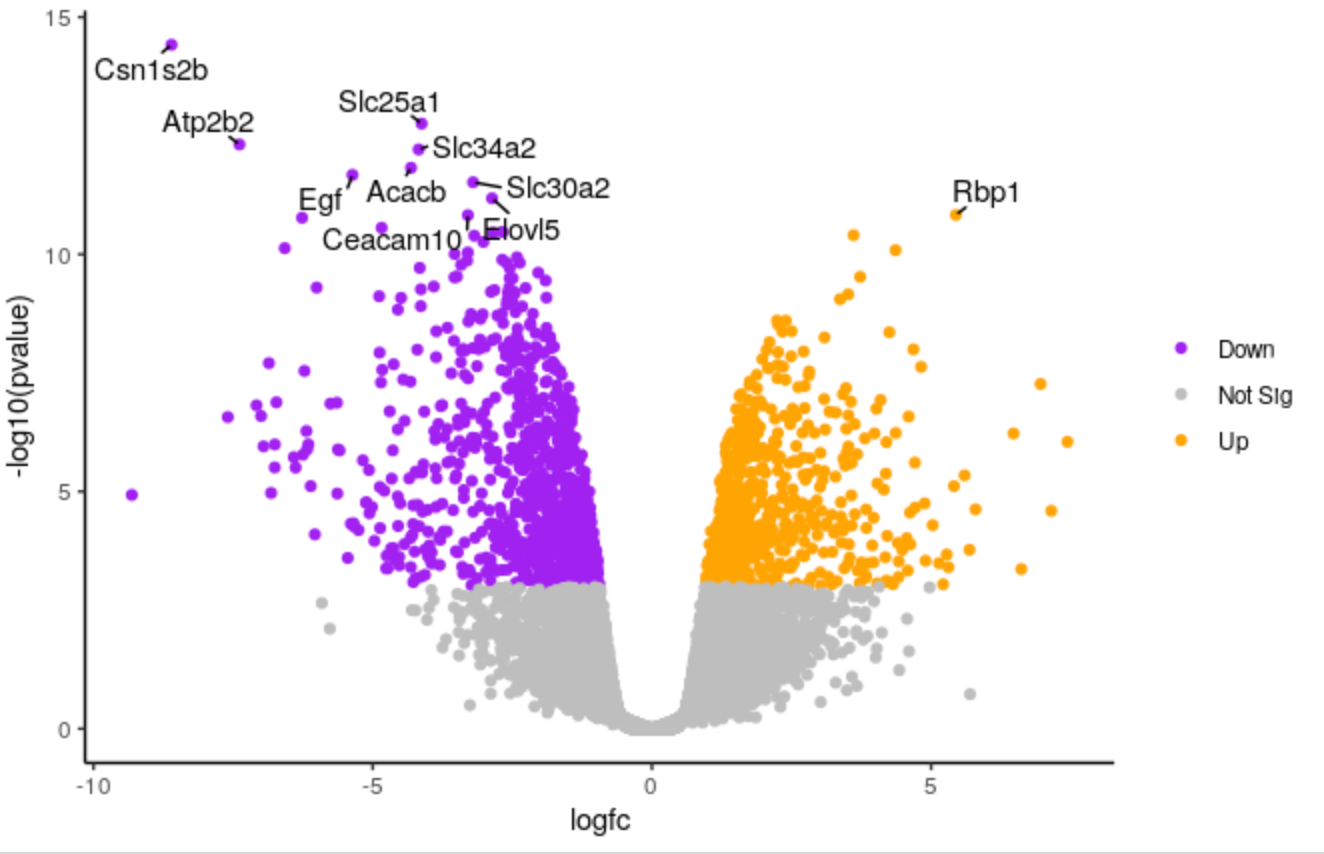
We’ll demonstate how you can change the colours. We’ll change the colour of the downregulated genes from cornflowerblue to purple. We’ll change the upregulated genes from firebrick to orange.
Hands-on: Change colours
Edit the line below in the script
# change the line
colours <- setNames(c("cornflowerblue", "grey", "firebrick"), c(down, notsig, up))

# to
colours <- setNames(c("purple", "grey", "orange"), c(down, notsig, up))
Highlight the code in the script and run
If you want to use other colours you can see the built-in R colours with their names in this cheatsheet.
Change points size
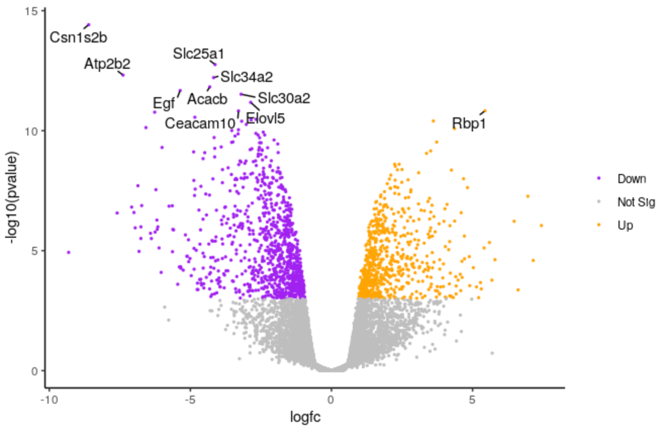
We’ll make the points a bit smaller. We’ll change to 0.5.
Hands-on: Change points size
Edit the line below in the script
# change the line
geom_point(aes(colour = sig)) +

# to
geom_point(aes(colour = sig), size = 0.5) +
Highlight the code in the script and run
QuestionHow could we change the transparency of the points?
We could use
alpha =. For examplegeom_point(aes(colour = sig), alpha = 0.5)
Change labels size
We’ll make the font size of the labels a bit smaller.
Hands-on: Change labels text size
Edit the line below in the script
# change the line
geom_text_repel(data = filter(results, labels != ""), aes(label = labels),

# to
geom_text_repel(data = filter(results, labels != ""), aes(label = labels), size = 3,
Highlight the code in the script and run
QuestionHow could we change the number of genes labelled from 10 to 20?
We could change the 10 to 20 here
top <- slice_min(results, order_by = pvalue, n = 20)
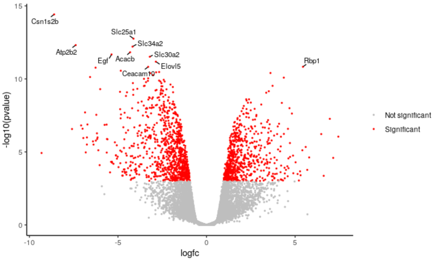
Change categories
We can change the categories of points we’re colouring in the plot. For example, instead of using separate categories for upregulated, downregulated we could just use a single category for significant.
Hands-on: Change categories
Change the category names to signif and notsignif
# change
down <- unlist(strsplit('Down,Not Sig,Up', split = ","))[1]
notsig <- unlist(strsplit('Down,Not Sig,Up', split = ","))[2]
up <- unlist(strsplit('Down,Not Sig,Up', split = ","))[3]

# to
signif <- "Significant"
notsignif <- "Not significant"
Specify which genes are signif and notsignif
# change
results <- mutate(results, sig = case_when(
                            fdr < 0.01 & logfc > 0.58 ~ up,
                            fdr < 0.01 & logfc < -0.58 ~ down,
                            TRUE ~ notsig))

# to
results <- mutate(results, sig = case_when(
                            fdr < 0.01 & abs(logfc) > 0.58 ~ signif, # abs() will give us absolute values i.e. all > 0.58 and < -0.58
                            TRUE ~ notsignif))
Specify the colours for signif and notsignif
# change
colours <- setNames(c("purple", "grey", "orange"), c(down, notsig, up))

# to
colours <- setNames(c("grey", "red"), c(notsignif, signif))
runHighlight the code in the script and
QuestionHow would you remove the legend from the plot? You can use Google.
If you Google
remove legend ggplot2you may find a few ways it can be done. One way isp <- p + theme(legend.position = "none")
You can save the edited script by clicking the galaxy-save icon at the top of the script in RStudio or through File > Save. You can download from Galaxy RStudio from the Files pane by ticking the box beside the script name, then More > Export > Download.
If you enter values in the Volcano Plot Galaxy tool form for Plot options, such as plot title, x and y axis labels or limits, they’ll be output in the script. This is one way you could see how to customise these options in the plot.
Conclusion
In this tutorial we have seen how a volcano plot can be generated and customised using Galaxy and R. You can see some more possible customisations in the RNA Seq Counts to Viz in R tutorial and at the ggrepel website.
Key points
R can be used to customise Volcano Plot output
The RStudio interactive tool can be used to run R inside Galaxy
Frequently Asked Questions
Have questions about this tutorial? Check out the tutorial FAQ page or the FAQ page for the Transcriptomics topic to see if your question is listed there. If not, please ask your question on the GTN Gitter Channel or the Galaxy Help ForumUseful literature
Further information, including links to documentation and original publications, regarding the tools, analysis techniques and the interpretation of results described in this tutorial can be found here.
Feedback
Did you use this material as an instructor? Feel free to give us feedback on how it went.
Did you use this material as a learner or student? Click the form below to leave feedback.
Citing this Tutorial
- Maria Doyle, Visualization of RNA-Seq results with Volcano Plot in R (Galaxy Training Materials). https://training.galaxyproject.org/training-material/topics/transcriptomics/tutorials/rna-seq-viz-with-volcanoplot-r/tutorial.html Online; accessed TODAY
- Hiltemann, Saskia, Rasche, Helena et al., 2023 Galaxy Training: A Powerful Framework for Teaching! PLOS Computational Biology 10.1371/journal.pcbi.1010752
- Batut et al., 2018 Community-Driven Data Analysis Training for Biology Cell Systems 10.1016/j.cels.2018.05.012
Congratulations on successfully completing this tutorial!@misc{transcriptomics-rna-seq-viz-with-volcanoplot-r, author = "Maria Doyle", title = "Visualization of RNA-Seq results with Volcano Plot in R (Galaxy Training Materials)", year = "", month = "", day = "" url = "\url{https://training.galaxyproject.org/training-material/topics/transcriptomics/tutorials/rna-seq-viz-with-volcanoplot-r/tutorial.html}", note = "[Online; accessed TODAY]" } @article{Hiltemann_2023, doi = {10.1371/journal.pcbi.1010752}, url = {https://doi.org/10.1371%2Fjournal.pcbi.1010752}, year = 2023, month = {jan}, publisher = {Public Library of Science ({PLoS})}, volume = {19}, number = {1}, pages = {e1010752}, author = {Saskia Hiltemann and Helena Rasche and Simon Gladman and Hans-Rudolf Hotz and Delphine Larivi{\`{e}}re and Daniel Blankenberg and Pratik D. Jagtap and Thomas Wollmann and Anthony Bretaudeau and Nadia Gou{\'{e}} and Timothy J. Griffin and Coline Royaux and Yvan Le Bras and Subina Mehta and Anna Syme and Frederik Coppens and Bert Droesbeke and Nicola Soranzo and Wendi Bacon and Fotis Psomopoulos and Crist{\'{o}}bal Gallardo-Alba and John Davis and Melanie Christine Föll and Matthias Fahrner and Maria A. Doyle and Beatriz Serrano-Solano and Anne Claire Fouilloux and Peter van Heusden and Wolfgang Maier and Dave Clements and Florian Heyl and Björn Grüning and B{\'{e}}r{\'{e}}nice Batut and}, editor = {Francis Ouellette}, title = {Galaxy Training: A powerful framework for teaching!}, journal = {PLoS Comput Biol} Computational Biology} }
You can use Ephemeris's
shed-tools installcommand to install the tools used in this tutorial.shed-tools install [-g GALAXY] [-a API_KEY] -t <(curl https://training.galaxyproject.org/training-material/api/topics/transcriptomics/tutorials/rna-seq-viz-with-volcanoplot-r/tutorial.json | jq .admin_install_yaml -r)Alternatively you can copy and paste the following YAML
---
install_tool_dependencies: true
install_repository_dependencies: true
install_resolver_dependencies: true
tools:
- name: volcanoplot
  owner: iuc
  revisions: 83c573f2e73c
  tool_panel_section_label: Graph/Display Data
  tool_shed_url: https://toolshed.g2.bx.psu.edu/